Transforming the Area under the Normal Curve (AUC) into Cohen’s d, Pearson’s r_pb, Odds-Ratio, and Natural Log Odds-Ratio: Two Conversion Tables

Introduction

Many research domains of life, social, and experimental sciences report their findings in terms of an effect size (ES) estimate. Nevertheless, there is not a single agreed definition of ES. In this regard, Kelley and Preacher (2012) revised several definitions of ES and provided a useful and comprehensive definition. According to Kelley and Preacher (2012, p. 140), ES is defined as “a quantitative reflection of the magnitude of some phenomenon that is used for the purpose of addressing a question of interest.” In this definition, an effect is a quantitative reflection of a phenomenon, and size is the magnitude of something.

The use of an ES was recommended by the American Psychological Association (APA) Task Force on Statistical Inference (Wilkinson, 1999). The Task Force (Wilkinson, 1999, p. 599) stressed that “reporting and interpreting effect sizes in the context of previously reported effects is essential to good research. It enables readers to evaluate the stability of results across samples, designs, and analyses.” Currently, this practice is also required by some editors and journals.

The number of ES measures is large, and the use of one or other coefficient depends, in part, on the traditions of a particular science or research area. The three most relevant factors for selecting a specific ES are: (a) the research question and the goals of the study; (b) the design type (e.g., experimental, correlational, cross-sectional, longitudinal, and so on), and (c) the nature of the variables and how they are measured (e.g., continuous, categorical, true dichotomous, dichotomized, and so on).

The most common ES estimates are the correlation coefficient (e.g., Pearson’s r), Cohen’s d, and z. Nevertheless, many other ES indexes are available to researchers. For example, ratios, odds-ratio (OR), natural log odds-ratio - ln(OR) -, relative operating characteristic (ROC) curves, among others, are used for reporting findings (see Borenstein, Hedges, Higgings, & Rothstein, 2009; Card, 2012; Cohen, 1977; Cooper, Hedges, & Valentine, 2009; Hedges & Olkin, 1985; Kelley & Preacher, 2012; Sánchez-Meca, Marín-Martínez, & Chacón- Moscoso, 2003; for a large variety of ES indexes). In the last thirty years, the importance of calculating and reporting ESs has increased as they are the basis for cumulative quantitative research and meta-analysis.

For example, the family of Pearson correlation coefficients is widely used in validity studies in work and organizational (W/O) psychology (e.g., Lado & Alonso, 2017; Rodríguez, 2016) and in psychometric meta-analytic methods and validity generalization studies (Salgado, 2017; Salgado, Moscoso, & Anderson, 2016; Schmidt & Hunter, 2015). Cohen’s d is the most common ES in experimental studies, for estimating the utility of clinical interventions (e.g., the effects of psychotherapy), in the Glassian meta-analytic method (Glass, 1976; Glass, McGraw, & Smith, 1981), and in the study of gender differences (e.g., Alonso & Moscoso, 2017; Alonso, Moscoso, & Salgado, 2017). Fisher’s Z transformation of correlation coefficients is used extensively in the study of attitudes and is the basis of the correlational meta-analysis method developed by Hedges and Olkin (1985). For its part, the area under the curve (AUC) is a relatively frequently used estimate of the effect size of the decisions taken under risk and uncertainty, in vigilance studies, forensic studies, law and human behavior studies, and, also, it is the basis for the estimates of the ROC curve when a normal distribution is assumed (Balaswany & Vardhan, 2015; Hasselblad & Hedges, 1995; Krzanowski & Hand, 2009; Marzban, 2004; Rice & Harris, 1995; Swets, 1973).

Nevertheless, even within these research areas and domains, despite the fact that a specific ES index is more frequently employed, empirical studies use a variety of them for reporting their findings. Due to this, over the years, some formulas have been developed for the conversion of one ES coefficient into others. For example, there are formulas for converting r into d, and r into z, and vice versa (see, for example, Rosenthal, 1991, for a large number of formulas). There are also a large number of mathematical functions for converting AUC into z, and vice versa (e.g., Brophy, 1983; 1985; Bryc, 2002; Choudhury, 2014; Emerson, 1979; Hart, 1957; 1966; Polya, 1945; Zelen & Severo, 1964). Consequently, it is also technically possible to transform, for instance, the AUC into Cohen’s d through several, successive intermediate conversions. These transformations are very useful and necessary from a practical point of view, as for both researchers and practitioners it is very convenient to have the possibility of unifying findings in a common metric unit. The transformations are also useful for meta-analysis, as these methods require the estimation of all the ESs using the same coefficient.

A problem with some empirical studies is that they do not inform about the ES and report the results in terms of alternative statistical coefficients, such as F, t, ², and so on. For this reason, researchers need to transform these values into an ES index. It is also important that researchers can transform the results reported in one metric into a different metric. For example, it is relatively common and easy for researchers to transform t, F, and ² into Pearson’s r or into Cohen’s d and Pearson’s r into Cohen’s d or Cohen’s d into Pearson’s r (see Rosenthal, 1991). However, the transformation is less common for other ES indexes, e.g., OR and Ln(OR), ratios, due mainly to two factors. One is the difficulty of the calculations. For, example some calculation involve logarithms, potencies, cosine values, etc. (see Bonnet, 2007, Hedges & Olkin, 1985; Salgado, 2016; for some examples). The second factor is that some formulas are relatively unknown (e.g., the formula for the standard error of a ratio, the formula for converting the point-biserial correlation, r_pb, into OR). For example, Block and Crain (2007) stated that no transformation existed for converting OR and relative risk (RR) into a correlation, but a formula suggested by Pearson (1900) is available (see Bonnet, 2007, for additional formulas). A third factor is that a number of published articles do not contain the data to calculate (or re-calculate) ESs. Moreover, the majority of well-known software is focused on the most typical ES indexes.

Therefore, converting one ES into another is technically possible and several transformation formulas are available to the researchers. However, many of these transformations require a number of intermediate conversions that increase the computational work of the researchers, together with the additional complication that many of the conversions are not available by default in the most popular statistical packages (e.g., SPSS, SAS). Furthermore, some of these intermediate transformations consist of large series of potencies. This difficulty has the side-effect that in meta-analytic studies some researchers exclude some primary studies from the final database because they cannot transform the original statistical coefficient into the effect size used in the meta-analytic method (typically, r and d in psychology, for instance).

The objective of this paper is to provide researchers and practitioners with tables for converting AUC-values into Cohen’s d, r_pb for different base rates, OR, and Ln(OR). At present researchers and practitioners have the possibility of using the Table constructed by Rice and Harris (2005), which gives the Cohen’s d and r_pb values for 137 AUC values. However, there are no Tables for converting the AUC-values directly into OR and Ln(OR) (and vice versa), nor are there for r_pb for base rates other than 50%.

ROC Area and Effect Sizes

In a pioneering effort, Rice and Harris (2005) posited the necessity of converting research results (e.g., F, and²) into ES and, particularly, they highlighted the importance of the area under the curve (AUC) as an index in forensic psychology research where it is commonly used. The area under the ROC curve is also frequently used in diagnostic areas (e.g., radiology, clinical microbiology) and in psychophysics, among other research and practice fields (see Swets, 1986b, for applications in different fields). For instance, Mossman (1994) illustrated its use in the study of violence and Humphryes and Swets (1991) showed its use for test validation purposes.

A ROC curve describes the functional relationships between the proportion of times that an alternative (say, h) is chosen when it occurs and the proportion of times that this alternative is chosen when another alternative (say, f) occurs. In signal-detection theory (SDT) terminology, h is termed hit rate (or success proportion, or true-positive proportion), and f is termed false-alarm rate (or failure proportion or false-positive proportion). The two most popular indices of discrimination are d and A_z, which describe how accurately experimental subjects and professionals perform a discrimination task (Swets, 1986a).

In the proposal of the index, Tanner and Swets (1954) defined d as the z score corresponding to f minus the z score corresponding to h, and it was termed index of detectability (Swets, 1986a). According to SDT, d is equal to the difference between the means of h and f distributions, expressed in standard deviation units of the f distribution (or equivalently for the standard deviation of the h distribution; see (Gescheider, 1976; Swets, 1986a). Therefore:

This equation shows the difference between the means of the two probability density functions (PDF) in terms of the standard deviation of the PDF for f (or, equivalently, for h). The d index assumes equal-variance normal distributions. However, as there are cases in which the assumption of equal variances is not held, an index termed Δm was proposed which is consistent with unequal-variance, normal distributions (Green & Swets, 1974; Gescheider, 1976; Swets, 1986a). The definition of Δm is similar to d, therefore,

It is obvious that if _h and_f are equal, then d´ and Δm are equal too. Interestingly, the Δm index is algebraically equivalent to the Δ coefficient given by (Glass 1976; Glass, McGraw, & Smith, 1981) for examining the effect of psychotherapy treatments. According to Glass et al. (1981), Δ is equal to the difference between the mean of the treatment group and the control group mean expressed in standard deviation units of the control group,

Therefore, Glass’ Δ and Δm are analogous. In addition, Glass’ Δ can be considered a special case of Cohen’s d, because if the standard deviation of the control group (_C) is equal to the standard deviation of the treatment group (_T), Cohen’s d and Glass’ Δ are equal, therefore d´, Δm, Glass’ Δ, and Cohen’s d are equal too. Otherwise, Cohen’s d can be smaller or larger than Glass’ Δ depending on the value of the ratio _T/_c. If the ratio is greater than 1, Cohen’s d will be larger than Glass’ Δ and if the ratio is smaller than 1, Cohen’s d will be smaller Glass’ Δ.

The second SDT index, A_z, was defined by Swets (1986a, p. 114) as the “area under the cumulative normal function up to the normal-deviate value equal to z(A)”. The A_z index can range from .5 to 1 and it assumes any form of distribution that can be transformed monotonically to the normal distribution (Swets, 1986a). Consequently, as A_z is the area under the normal curve, if the two variances are equal, Swets, (1986a, equation 21) showed that

and, therefore, if the two variances are unequal

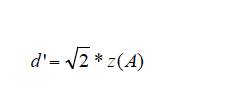
These last two equations are particularly relevant because, due the equivalence among d´, Δm, Glass’ Δ, and Cohen’s d shown above, they provide a way to transform the AUC into a Cohen’s d. In addition, as Hedges and Olkin (1985) suggested, the assumption of equal population variances is reasonable in many cases in life and social sciences.

A point that must be mentioned is that, in some cases, the observed A_z values are underestimates of the true A_z (Humphreys & Swets, 1991; Swets, 1986b). This is due to the fact that they were computed on a selected sample of individuals. For example, only the subgroup of most violent individuals, and not all the violent individuals within the group attending a psychotherapy program, the first sub-group will be restricted (selected). The same would happen if only a selected group of candidates takes a training course. This selection bias causes the standard deviation of this restricted group to be smaller than the standard deviation of the large group. Therefore, in some cases, the inequality of variances between the two distributions can be, in part, due to the artefactual effects of the selection bias and not because there is a true inequality. Gray, Begg, and Greenes (1984) developed an approach to correct A_z for selection bias.

In order to facilitate comparisons across follow-up studies that report different ES indexes, Rice and Harris (2005) developed a table of the equivalences among AUC and d, and r_pb. Rice and Harris (2005) Table includes the AUC values from .50 to 1 and the respective values of z, d, and r_pb. One limitation of Rice & Harris’ Table is that it includes values for a 50% base rate only. In other words, p = q = .5. However, base rates different from 50% are not uncommon in practice and research (Swets, Dawes, & Monahan, 2000). The base rate is important because the r_pb value corresponding to a specific d value depends partially on the base rate. Therefore, for the same d value, different r_pb can exist depending on the base rate. Moreover, as soon the base rate differs from 50%, the r_pb values decrease, so the larger (or smaller) than 50% the base rate, the smaller the r_pb.

To create the Table, Rice and Harris used three types of information. First, they converted the AUC values into z-scores (or normal deviate of AUC), using the Tables of Pearson and Hartley (1954). Second, they used the formula to transform the z-value into a Cohen’s d value as mentioned above:

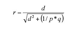
Next, to transform the Cohen’s d value into the equivalent r_pb value, they used the well-known formula:

On this point, it is important to take into account that the conversion of d to a correlation is always r_pb, but this is true only when a true binary variable is used in the study. In other words, the nature of the dichotomization must be considered. If the dichotomization is natural (e.g., treatment vs. non-treatment; men vs. women), then the conversion from d produces r_pb, but if the dichotomization is artificial (i.e., a continuous variable is divided into two groups), then the conversion of d is an underestimation of r. Hunter and Schmidt (1990, p. 276) suggested a process to convert from d to Pearson’s r if the binary variable is a result of an artificial dichotomization: d would first convert to r_pb and, then, it would convert from r_pb to r. This clarification is relevant because as Nunnally (1978), among others stated, if a continuous variable is split into two values (or groups), the maximum value of correlation is not 1, but rather .79 (when p = q = .50, otherwise it is lower than .79). A detailed account of this issue appears in Hunter and Schmidt (1990, chapters 3 and 6). Moreover, if a correlational study was done with two continuous variables and the researcher’s goal is to transform the r into a Cohen’s d, such Pearson’s r can be directly transformed into a Cohen’s d.

Consequently, the d values under the first research design (i.e., true experiment, true binary variable) and the second one (i.e., artificial dichotomization of a continuous variable) provide different information and different estimates of the ES. For example, a Pearson’s r of .50 equals an r_pb of .40 (for p = q = .50) and equals a d of .87.

When a continuous variable is dichotomized, r_pb underestimates r by a factor of y/√(p*q), where p*q is the standard deviation of X (p = proportion of cases in the higher group or hits and q = 1 - p) and y is the ordinate of the normal-distribution curve at the point of division between p and q. The underestimation varies from about 1.25 when p = .5 to about 3.73 when p = .99 (Guilford & Fruchter, 1978, p. 311; Hunter & Schmidt, 1990, p. 256; see also Magnusson, 1967).

Aims of This Study

Two new extended Tables have been created using a process of six steps. In each step, a new transformation of the AUC is made and a different ES estimate is given. In addition to z, the new Tables provide the estimates of AUC as Cohen’s d for dichotomous variables, r_pb, OR, and the Ln(OR) for continuous and dichotomous variables.

The process of construction of Table 1 was as follows. The first step was the conversion of an AUC-value into a z coefficient. This conversion can be made using the following equation provided by Zelen and Severo (1964, p. 933):

Where

Or it can be made using one of the functions listed by Yerukala and Boiroju (2015), all of which produce practically identical values until the third decimal. The second step was to convert the z-value into a Cohen’s d, using the formula given by Swets (1986a):

The third step involved the conversion of a Cohen’s d into an r_pb. This was done for base rates of .5, .3, .2, and .1. The equation is:

Where K = 1/p*q. Therefore, K values for p = 5, .3, .2, and .1 are, 4, 4.76, 6.25, and 11.11, respectively. The K values clearly illustrate the decline of the r_pb as the p values decrease.

Table 2 provides the d-values converted to OR and Ln(OR). The construction of Table 2 followed the same first two steps used for Table 1. The third step for Table 2 was to use the next two equations, provided by Borenstein et al. (2009), Card (2012), Hasselblad and Hedges (1995), and Sánchez-Meca et al. (2003) for obtaining the respective values of Ln(OR) and OR. These formulas are:

and

In summary, Table 1 provides the values for the conversion from AUC to z, d-Cohen, and r_pb, for four base rates, and Table 2 provides the values for the conversion from AUC to z, d-Cohen, Ln(OR), and OR.

Conclusion

Reporting ESs is a more and more common practice in research and Pearson’s r and Cohen’s d are two of the most frequently used indices of ES. However, a large variety of ES indices are used. Some of them are particularly used in specific research domains. The AUC is one of the most typically reported in forensic psychology research and in diagnostic and clinical research (e.g., radiology). Odds-ratio (OR) and its varieties - e.g., Ln(OR), risk ratio - are also commonly found in articles reporting research findings. To encourage applied and forensic psychology researchers to report an ES and also the conversion of a variety of ES indices to a common metric, this article tabulated the conversion from AUC into Cohen’s d, OR, Ln(OR), and r_pb for base rates of 50%, 30% 20% and 10% for 500 AUC three-digit values. Rice and Harris’ (2005) Table does not provide r_pb values for base rates other than 50% nor for ESs other than Cohen’s d and r_pb. Therefore, the new tables can be seen, to a certain extent, as an extension of Rice and Harris’s Table.

Researchers should be aware of when it is correct and appropriate to transform a specific ES into another one and when the transformation is not appropriate, even when the formulas can be used in both cases. For example, d’ should not be transformed into OR when a within-group design is used, as OR requires a design with two independent samples. With regard to Cohen’s d transformation into a correlation coefficient, the nature (true binary vs. dichotomized) of the independent variable dictates what type of correlation coefficient should be obtained (see pages 10-11). Therefore, we recommend the researchers make a reasonable use of the transformation formulas.

In summary, this article presents two new Tables for obtaining four types of ESs from AUC-values and, simultaneously, converting an ES index in several others. In addition, researchers and practitioners can calculate by themselves the ES of interest with the formulas included here for the values not given in the Tables.