
Decoding Artificial Intelligence: A Tutorial on Neural Networks in Behavioral Research
[Decodificando la inteligencia artificial: Un tutorial sobre redes neuronales en las Ciencias del Comportamiento]
Javier Martínez-García2, Juan José Montaño1, 2, Rafael Jiménez1, 2, Elena Gervilla1, 2, Berta Cajal1, 2, Antonio Núñez1, 2, Federico Leguizamo1, 2, Albert Sesé1, and 2
1University of the Balearic Islands, Palma, Balearic Islands, Spain; 2PSICOMEST Research Group, Health Research Institute of the Balearic Islands (IdISBa), Palma, Balearic Islands, Spain
https://doi.org/10.5093/clh2025a13
Received 21 February 2025, Accepted 31 March 2025
Abstract
Background: Artificial Neural Networks (ANNs), particularly multilayer perceptrons (MLPs) with backpropagation, are increasingly used in Behavioral and Health Sciences for data analysis. This paper provides a comprehensive tutorial on implementing backpropagation in MLP models for regression and classification tasks using Python. Method: The tutorial guides readers step-by-step through building a backpropagation MLP using a simulated data matrix (N = 1,000) with psychological variables, demonstrating ANNs’ versatility in predicting continuous variables and classifying (binary and polytomous) patterns. Python scripts and detailed output interpretations are included. Results: MLP models trained with backpropagation show effectiveness in regression (R² = .71) and classification (binary AUC = .93, polytomous AUC range: .81-.93) on test sets. Conclusions: This tutorial aims to demystify ANNs and promote their use in Behavioral and Health Sciences and other fields, bridging the gap between theory and practical implementation.
Resumen
Introducción: Las Redes Neuronales Artificiales (RNA), especialmente los perceptrones multicapa (MLPs) con retropropagación, son cada vez más utilizadas en Ciencias del Comportamiento y de la Salud para analizar datos. Este artículo presenta un tutorial completo sobre la implementación de modelos MLP con retropropagación para tareas de regresión y clasificación usando Python. Método: El tutorial guía paso a paso la construcción de un MLP con retropropagación utilizando una matriz de datos simulados (N = 1,000) con variables psicológicas, demostrando la versatilidad de las RNA en la predicción de variables continuas y clasificación de (binarios y politómicos). Se incluyen scripts de Python y su interpretación detallada. Resultados: Los modelos MLP muestran eficacia en regresión (R² = 0.71) y clasificación (AUC binaria = .93, rango AUC politómica: .81-.93) en los tests. Conclusiones: Este tutorial persigue desmitificar las RNA y promover su uso en Ciencias del Comportamiento y la Salud, facilitando la transición de la teoría a la práctica.
Palabras clave
Inteligencia artificial, Redes neuronales artificiales, PerceptrĂłn multicapa, Algoritmo de retropropagaciĂłn, Python, Ciencias del comportamiento y de la saludKeywords
Artificial intelligence, Artificial neural networks, Multilayer perceptron, Backpropagation algorithm, Python, Behavioral and health sciencesCite this article as: Martínez-García, J., Montaño, J. J., Jiménez, R., Gervilla, E., Cajal, B., Núñez, A., Leguizamo, F., and Sesé, A. (2025). Decoding Artificial Intelligence: A Tutorial on Neural Networks in Behavioral Research. Clinical and Health, 36(2), 77 - 95. https://doi.org/10.5093/clh2025a13
Correspondence: juanjo.montano@uib.es (J. J. Montaño Moreno).Artificial Neural Networks (ANNs) have emerged as the cornerstone of modern Artificial Intelligence (AI), revolutionizing the field and enabling unprecedented advancements in machine learning and cognitive computing. These computational models, inspired by the biological neural networks found in animal brains, form the foundation upon which many of today’s most sophisticated AI systems are built. By mimicking the interconnected structure of neurons and synapses, ANNs have demonstrated remarkable capabilities in pattern recognition, decision-making, and complex problem-solving across a wide array of domains. As the driving force behind deep learning algorithms, ANNs have become instrumental in pushing the boundaries of AI, from natural language processing and computer vision to autonomous systems and predictive analytics. The impact of ANNs and AI extends far beyond traditional computer Science applications, finding increasing relevance in the realm of behavioral Sciences. As researchers seek to unravel the complexities of human behavior, cognition, and social interactions, these advanced computational tools offer new avenues for analysis and prediction. Moreover, recent studies have shown that machine learning algorithms can effectively analyze complex behavioral data to uncover intricate patterns related to psychological well-being and decision-making processes, demonstrating the power of AI in identifying and understanding multifaceted psychological issues (Vezzoli & Zogmaister, 2023). The ability of ANNs to process high-dimensional data allows researchers to explore complex relationships among various psychological constructs, thereby addressing limitations inherent in traditional statistical methods. This capability is particularly significant in understanding mental health issues where interactions among biological, emotional, cognitive, and environmental factors are critical. Thus, ANNs are being of great use in modeling and understanding cognitive processes such as the learning of abstract concepts (Piloto et al., 2022; Roads & Mozer, 2021), the production and understanding of natural language (Arana et al., 2024), the detection of emotional patterns from facial recognition (Faltyn et al., 2023; Song, 2021; Wei et al., 2021) or from written language (Qamar et al., 2021). In the field of clinical psychology, these techniques have been used in the detection of internet users with suicidal intentions (Schoene et al., 2023), the prediction of maladaptive behaviors (low academic performance, drug use, delinquency, etc.) (McKee et al., 2022) or in the identification of the optimal psychological treatment according to the patient’s characteristics (Hollon et al., 2019). Developmental and educational psychology has also benefited from the use of ANNs in the detection of autism through language (Wawer & Chojnicka, 2022), in the prediction of emotional and behavioral risk status in children (Wang et al., 2021) or in identifying student satisfaction with different learning modalities (Ho et al., 2021). Finally, the application of ANNs in the field of social psychology has focused in the detection of consumer needs and behavior towards product features (Barnes, 2022; Li et al., 2024), predicting the use of social networks (Ramírez et al., 2021) or in identifying the effects of social comparison among social network users (Jabłońska & Zajdel, 2020). As can be observed, the application of AI methodologies in Behavioral, Social, and Health Sciences is rapidly expanding, with potential uses ranging from diagnosis and prediction to understanding human development and functioning (Hassani et al., 2020). By harnessing the strengths of ANNs, researchers can gain deeper insights into human behavior and cognition, paving the way for innovative approaches to psychological assessment and intervention. The Multilayer Perceptron (MLP) and the Backpropagation Learning Algorithm: The Most Prevalent ANN There are currently many ANN models that are used in various fields of application in data analysis. Among these models, one of the most widely used is the multilayer perceptron (MLP) associated with the backpropagation error learning algorithm (Henninger et al., 2023), also called backpropagation network (Rumelhart et al., 1986). The main virtue of a MLP network that explains its widespread use in the field of data analysis is that it is a universal function approximator. The mathematical basis for this statement is due to Kolmogorov (1957), who found that a continuous function of different variables can be represented by the concatenation of several continuous functions of the same variable. This means that a perceptron containing at least one hidden layer with enough non-linear units could learn virtually any kind of relation if it can be approximated in terms of a continuous function (Hornik et. al., 1989). The backpropagation algorithm or one of its variants forms the basis of today’s deep learning in ANN models such as Long Short Term Memory (LSTM) (backpropagation through time) (Hochreiter & Schmidhuber, 1997), Convolutional Neural Networks (CNN) (LeCun et al., 1998), Deep Belief Networks (DBN) (Hinton et al., 2006), or Generative Adversarial Networks (GAN) (Goodfellow et al, 2014). The aim of this paper is to provide a tutorial for introducing researchers in the Behavioral and Health Sciences to the use of ANNs. This tutorial focuses on both regression (continuous outcomes) and classificatory (categorical outcomes: binary and polytomous) ANNs applications. To accomplish this goal, we present a step-by-step methodology for applying MLP with the backpropagation algorithm. We also provide a Python script that enables its implementation, utilizing the data described in the Dataset Generation subsection for regression and classification tasks. The script is designed for easy adaptation to any dataset involving regression or classification problems. Our aim is to make this resource valuable for researchers across various disciplines, enabling them to readily incorporate ANNs into their respective fields of study. A simulated dataset was created to embrace the relationships among psychological and demographic variables that influence psychological wellbeing, the primary outcome variable, in a sample of 1,000 individuals. The predictor variables consisted of gender (50.7% female), age (ranging from 18 to 85 years, mean = 51.63, Mdn = 52, SD = 17.11), and socioeconomic status, categorized as low (n = 343), medium (n = 347), and high (n = 310). Additional predictors included emotional intelligence (range: 24-120, M = 71.97, Mdn = 71, SD = 23.79), resilience (range: 4-20, M = 11.93, Mdn = 12, SD = 4.46), life satisfaction (range: 5-35, M = 20.09, median = 20, SD = 7.42), and depression (range: 0-63, M = 31.45, median = 32, SD = 14.85). The primary outcome variable was emotional wellbeing, measured on a scale from 0 to 100 (M = 50.22, Mdn = 49, SD = 24.45). The correlations established among these variables served as conditions for the simulation: psychological wellbeing was positively correlated with emotional intelligence (.50), resilience (.40), and life satisfaction (.60), indicating that higher levels of these factors were associated with improved emotional health outcomes. Conversely, a strong negative correlation existed between depression and psychological wellbeing (-.80), suggesting that higher depression scores were linked to lower emotional wellbeing. The variable age showed a slight positive correlation with emotional wellbeing (.15), reflecting the expectation that older individuals might experience greater emotional stability. Although gender and socioeconomic status were included as potential predictors, the simulation assumed no statistically significant differences in psychological wellbeing. The Welch’s t-test indicated no significant difference between females and males, t(989.88) = -0.93, p = .35. A one-way ANOVA on socioeconomic status also showed no significant differences in emotional wellbeing, F(2, 997) = 0.11, p = .90. Additionally, the dataset included categorical transformations of psychological wellbeing into binary and polytomous formats: a binary version (low = 477, high = 523) and a polytomous version with four levels: low (n = 161), somewhat (n = 351), quite a bit (n = 330), and very much (n = 158). The polytomous transformation used the 25th, 50th, and 75th percentiles to define the thresholds for categorizing psychological wellbeing scores. These transformations enabled analyses using MLP models for both regression (continuous outcome) and classification (categorical outcomes) tasks. The dataset can be downloaded in excel format here: Dataset (link 1). This tutorial focuses on Python, a language that has gained significant popularity in the Data Science industry over the past decade. Python’s appeal stems from its simplicity, versatility, and extensive ecosystem of tools and libraries tailored for data analysis, visualization, and machine learning. It provides a high-level interface for libraries written in performance-optimized languages like C++, while maintaining a simple syntax. This combination allows deep learning frameworks such as TensorFlow to leverage Python’s user-friendly nature while delegating computationally intensive tasks to optimized backends. Given that this tutorial is designed for researchers new to ANNs, we have prepared a preliminaries document explaining how to install and use the Anaconda platform and Jupyter Notebook. We will use Anaconda and Jupyter Notebook to run Python scripts, providing an interactive environment for writing and testing code. This document includes a step-by-step guide for setting up the applications and introduces basic Python programming for statistical modeling. It also includes a multiple regression analysis using the simulated matrix described earlier. The preliminaries document can be downloaded here: Preliminaries document (link 2). Steps in the Application of an MLP in Regression and Classification Tasks This subsection presents a step-by-step methodology for implementing a MLP with the backpropagation algorithm. We provide a Python script for this implementation, using the simulated matrix subsection for regression and classification tasks. For a comprehensive explanation of the MLP and backpropagation algorithm, along with practical tips for their application, the reader can download a technical document Methodology and practical tips in the application of a multilayer perceptron, in the following link: Introduction to MLP (link 3). At this point, it is assumed that the reader has already installed the Anaconda distribution and Jupyter Notebook to proceed with estimating an ANN model. We also assume that the reader has carefully reviewed the preliminaries document and has successfully completed a multiple regression model as a preparatory exercise. With that foundation in place, let’s now get started on applying ANN models. The script begins by importing essential libraries. We will use “numpy” for numerical operations and array handling, and “pandas” for managing DataFrames; “tensorflow” and “Keras” will be employed to build and train the neural network models. “Matplotlib” will then be used to generate plots and visualizations. The script also imports “shutil” for file operations and “pathlib” for working with files and directories. For evaluating model performance, different functions and options of “scikit-learn” library provides various metrics and model selection tools. Finally, “keras_tuner”, including HyperModel and BayesianOptimization, is included for hyperparameter tuning (Figure 1). Figure 1 Importing Required Libraries. 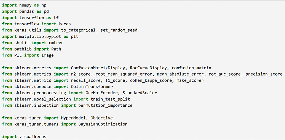 Calling the Data Matrix and Selection of Variables First, we set the random seed for reproducibility using Keras. Then, we import the dataset using Pandas, creating a DataFrame. Next, we convert categorical feature columns to the Category data type. We then separate the target features into dedicated variables and create the input features by dropping the target features from the DataFrame. This prepares the data for subsequent modeling. Note that the following script includes data preprocessing to simultaneously analyze the three tasks for which we will use the ANN: regression (with the Psychological Well-being variable in continuous format), binary classification (with the dichotomized Psychological Well-being variable, and multi-class classification (with the Psychological Well-being variable categorized into four classes). This is intended to illustrate the MLP’s ability to perform all three tasks in a didactic manner. Please, note that the script differentiates between the three tasks so the user can customize the analysis by selecting only one of them for their research purposes, based on the type of outcome variable they are using (Figure 2). Figure 2 Reading Data Matrix and Selecting Output Features for Each Task. 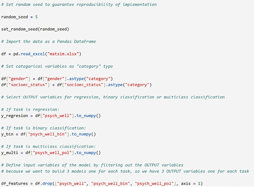 Creation of Training, Validation and Test Sets A common task in machine learning research is splitting the dataset into training and testing subsets. Splitting data into training and testing sets is essential to avoid overfitting, which can lead to an overestimation of a model’s performance. This involves passing the feature matrix and target variable, defining the test set size, and setting a random seed for reproducible splits. This approach provides a more accurate measure of how well our model generalizes to new, unseen data (Figure 3). Figure 3 Splitting Data into Training and Testing Sets. 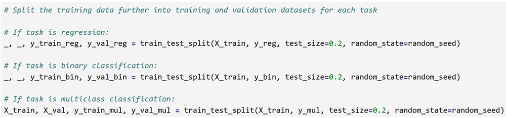 Additionally, to optimize hyperparameters, we split the training data into final training and validation sets. The final training set will fit the model’s parameters, while the validation set will guide hyperparameter tuning. This ensures the test set remains untouched, providing an unbiased evaluation of the model’s generalization capability (Figure 4). Figure 4 Splitting Training set into Training and Validation Sets. 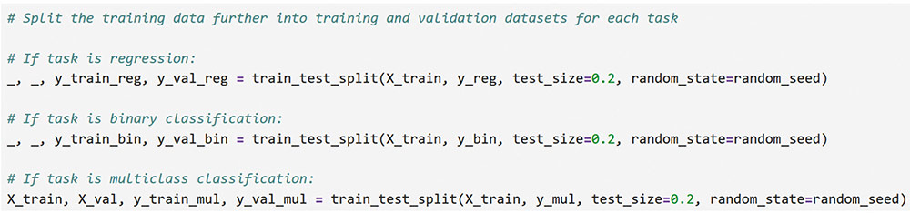 Neural networks typically require input data to be preprocessed. This often involves encoding categorical features, since neural networks work best with numerical data. We use OneHotEncoder from scikit-learn to perform dummy encoding, converting categorical columns into numerical representations. Additionally, continuous features are often standardized, and we use StandardScaler to achieve this. To streamline these preprocessing steps, we combine them into a single ColumnTransformer pipeline. This allows us to apply OneHotEncoder to categorical columns and StandardScaler to numerical columns within the same workflow. Crucially, the ColumnTransformer is fit “only” on the training data. This prevents data leakage, where information from the validation or test sets inadvertently influences the training process. After fitting, the preprocessor is then applied to all datasets (training, validation, and testing) to ensure consistent transformations (Figure 5). Figure 5 Performing Preprocessing Step on the Input Features. 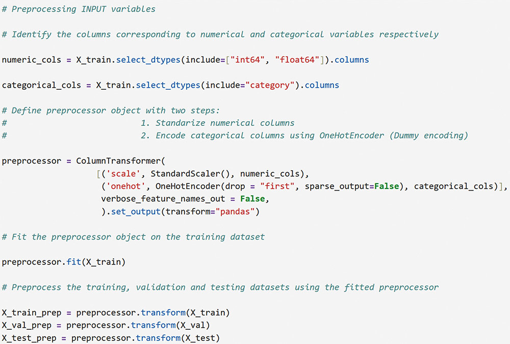 We will also need to preprocess our categorical output features. We also preprocess categorical output features or target variables. For binary targets, we encode classes as 0 and 1. For multiclass targets, OneHotEncoder transforms the target variable into a one-hot encoded vector, representing the correct class with a 1 and others with 0. Fitting the OneHotEncoder to the target values ensures consistent encoding across all datasets, preparing the output features for classification models (Figure 6). Figure 6 Encoding Output features for Classification Tasks. 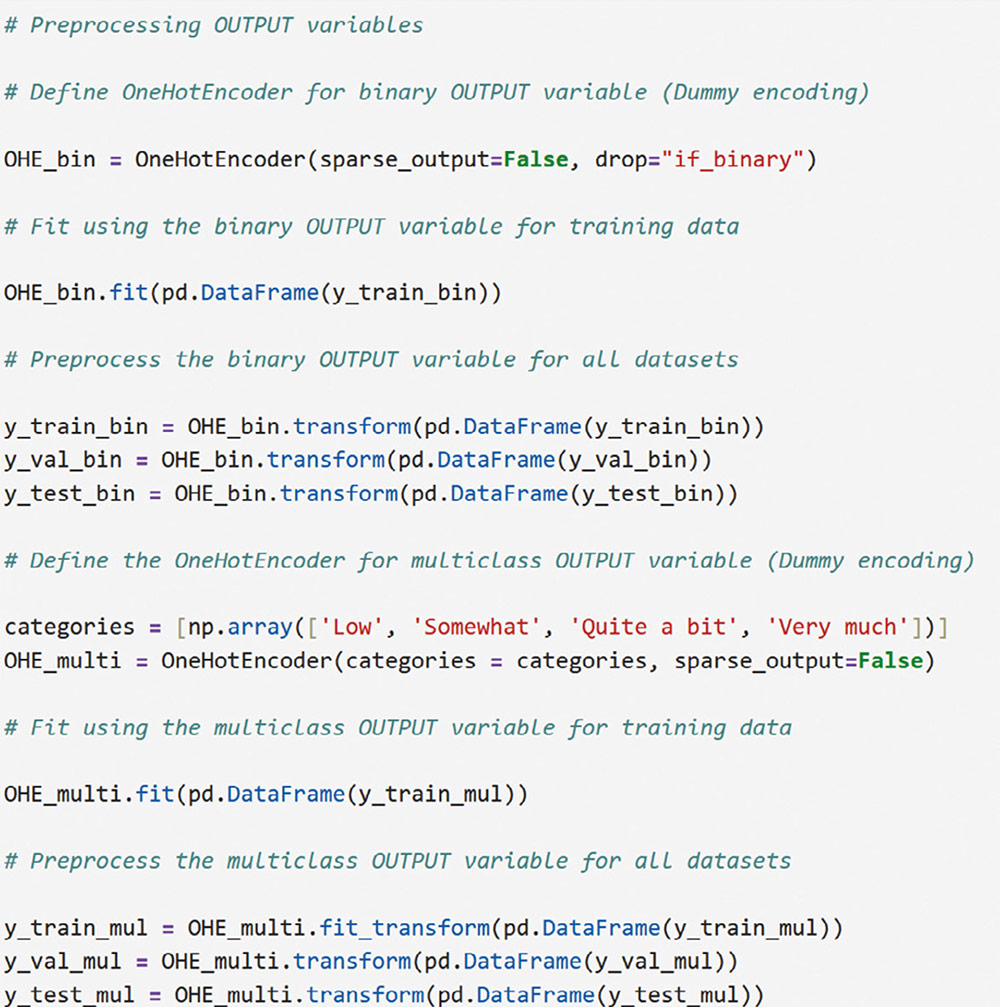 We create a template class for neural network models using the Keras library. The class requires a “method” parameter (regression, binary, or multiclass classification) to specify the problem type. The Keras Sequential API simplifies model building with automatic differentiation. We define hyperparameters using the keras-tuner library, “tuning” “float”, “int”, or “categorical values” during the hyperparameter tuning process. The following script shows the code for the MyHyperModel class, which inherits from Keras’ HyperModel and defines the build method. The build method defines hyperparameters like the number of neurons, learning rate, activation function, number of hidden layers, and regularizer. The model is built using the Keras Sequential API using these hyperparameters. Depending on the “method” specified, the appropriate output layer and loss function are selected for regression, binary classification, or multiclass classification. Finally, the Adam optimizer is defined, and the model is compiled. Finally, example models are created for regression, binary classification, and multiclass classification tasks (Figure 7). Figure 7 Creating Neural Network Models for Each Task Using MyHyperModel Class. 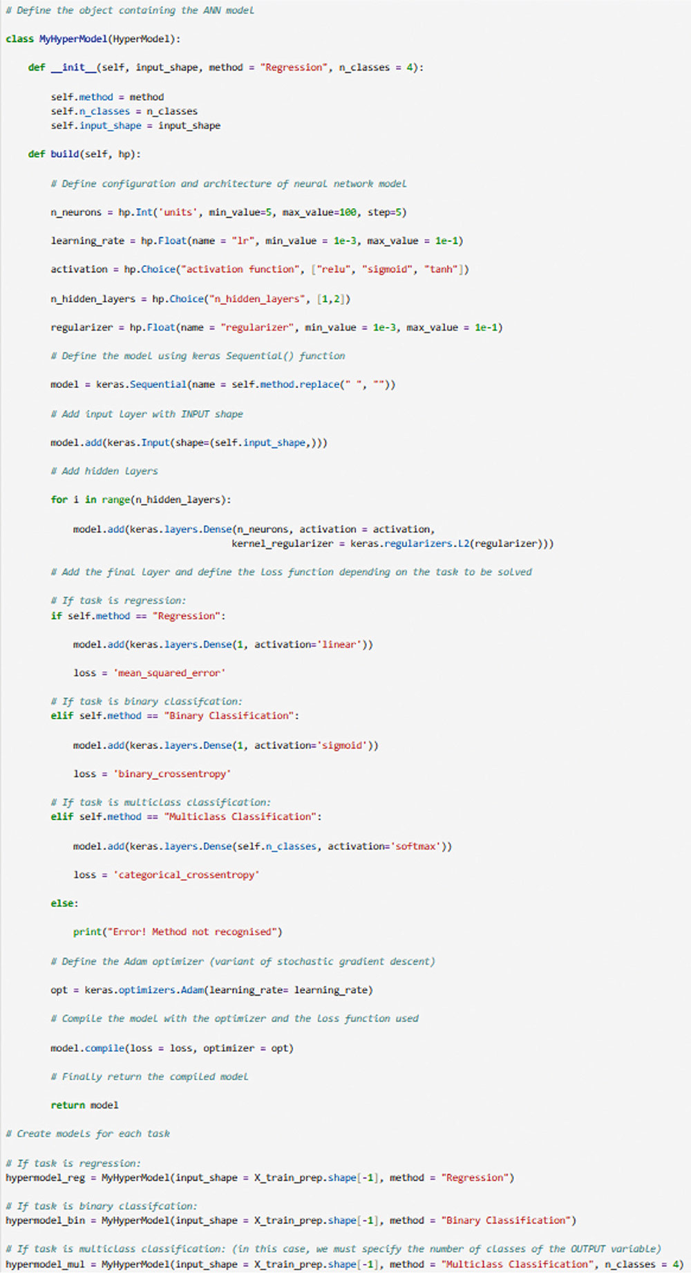 Choice of Initial Weights When a neural network starts learning, its “weights” are like initial guesses. Good starting guesses help it learn faster. The code uses a standard method for setting these initial guesses (called GlorotUniform), however, the MyHyperModel makes it easy to adjust the initial weights in the hidden layers through the kernel_initializer. Other options can be configured, but GlorotUniform is a sensible default to use, and the code will optimize it with the tool Keras Tuner. MLP Architecture The code builds an MLP, which can be seen as a team working together. The input and output are dictated by the data, but the number of hidden layers and the number of neurons (team members) needs to be decided. The number of hidden layers and neurons is crucial, the “n_hidden_layers” which in this case can be only 1 or 2, and the “n_neurons”, which can be from 5 to 100 with steps of 5, as it is defined in the picture of the script. Choosing the right number of hidden layers is a tradeoff, this are tunable values for the Keras Tuner tool. Learning Rate and Momentum Factor The learning rate is how quickly the model updates its knowledge. The MyHyperModel code uses an “Adam optimizer” that automatically adjusts the learning rate as training progresses. If the “learning_rate” is too big, the model will probably never learn, but if it is too small, it will take very long. In our case, we let the Keras Tuner tool tune the “learning_rate” with values that go from .001 (1e-3) to 0.1 (1e-1), as we can see in the script. Activation Function of the Hidden and Output Neurons The activation function of the hidden neurons introduces non-linearity, enabling the network to learn and approximate complex functions. Without activation functions, the network would behave like a linear model, regardless of the number of layers. In our case we will chose between logistic, hyperbolic tangent and ReLU functions (see Supplementary Material for further details). Figure 8 Performing Hyperparameter Tuning for Each Task. 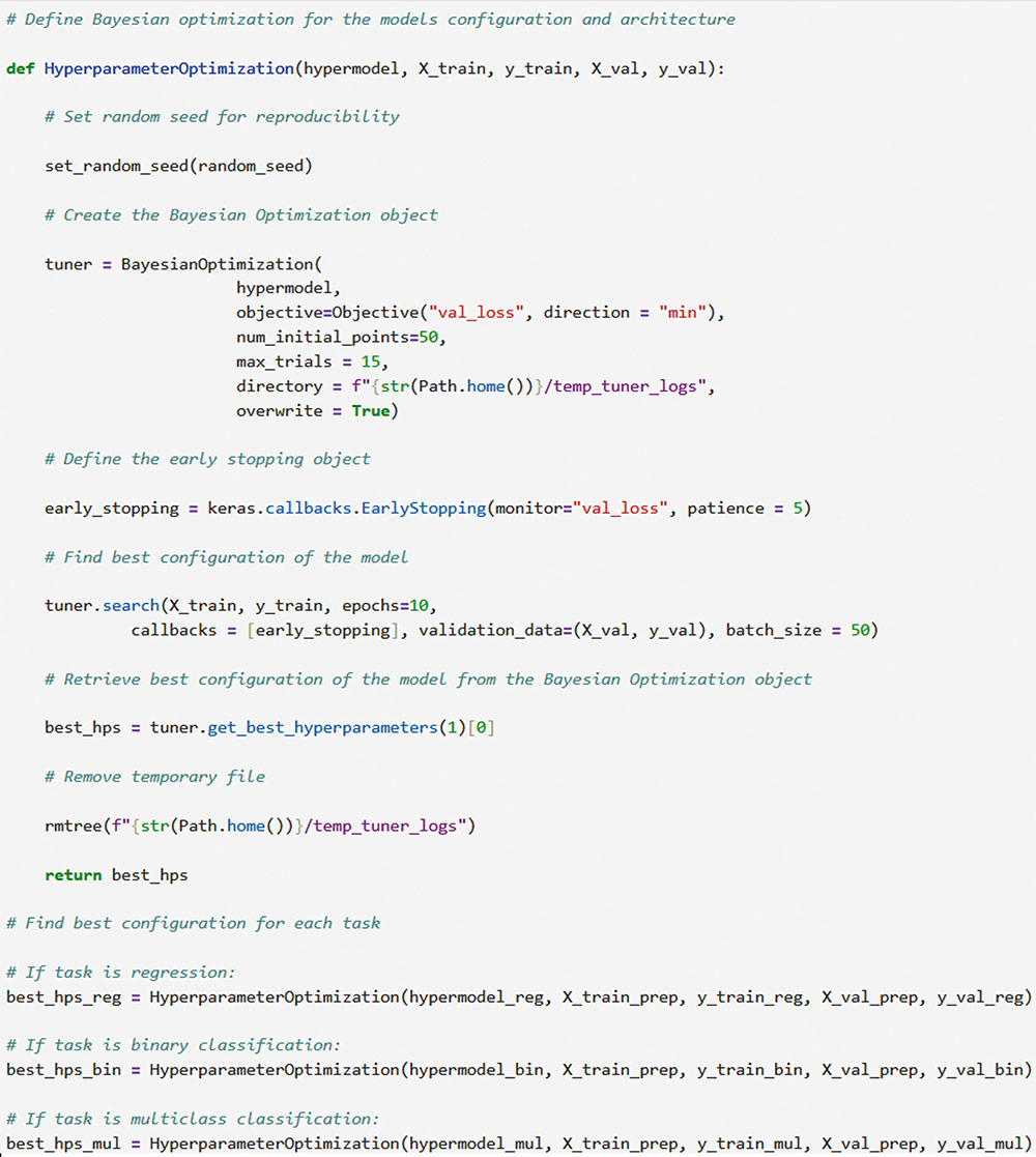 The activation function of the output neuron will depend on the task being performed. In the case of regression, a linear function will be used while in binary and multiclass classification a sigmoid and softmax functions will be used respectively to interpret the result as a probability. Model Definition and Compilation To begin, the model is defined using Keras’ Sequential function. Layers are added one by one. The first layer is the input layer, with neurons matching the input features (using InputLayer). Subsequent layers are fully connected (Dense), with neuron count and activation specified by hyperparameters. The output layer’s activation and neuron count depend on the problem type (the method parameter): linear for regression, sigmoid for binary classification, softmax for multiclass. The Adam optimizer is used for training, and the model is compiled with the optimizer and appropriate loss function (mean squared error for regression, binary/categorical cross-entropy for binary/multiclass, respectively). Finally, the model is created for each task by specifying the method parameter. Hyperparameter Tuning To train the model, we tune hyperparameters for best performance. Instead of manually trying all combinations, we use Bayesian optimization, a smart search method. To avoid overfitting, we use the validation loss (performance on data the model has not seen) to measure model quality, not the training loss. We also use early stopping: if the validation loss stops improving, we halt training. We define a function that sets up this Bayesian optimization tuner, embeds the model within, and includes early stopping. This function uses training and validation data, the early stopping configuration, sets maximum epochs, and sets the training batch size. The function searches for the best hyperparameters and returns them for the model. The following script includes the Bayesian optimization for the models’ configuration and architecture (Figure 8). When this script is executed, the MLP identifies the optimal parameters for each of the three models, which configure the final model to be trained in the next step. The parameter identification process generates an iterative output on the screen, concluding in several minutes, depending on the processor employed. After identifying the optimal set of hyperparameters, we can now train our final optimized model. We define a function that takes a given model, its set of optimized hyperparameters, and both the training and validation data to perform the training. This function instantiates our final model using the build method on our hypermodel object with the optimized hyperparameters. It also defines an early stopping object and trains the model using the fit method. Finally, the function returns the trained model to the user. We can then train our final models by passing the appropriate set of hyperparameters and data to this defined function. The training process of the final models spends a few seconds (Figure 9). Figure 9 Final Training Using the Best Hyperparameter Configuration. 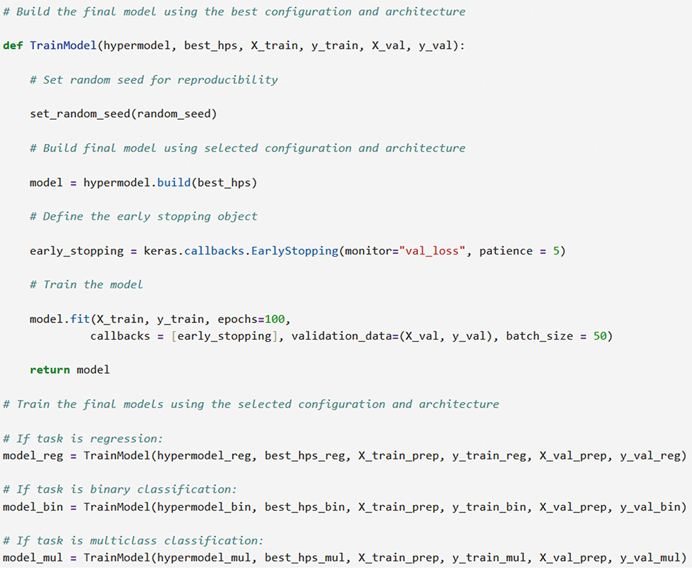 The following script displays the model configuration and the MLP architecture after training the selected model for each task (Figure 10). Figure 10 Plotting Neural Network Architecture for Each Task. 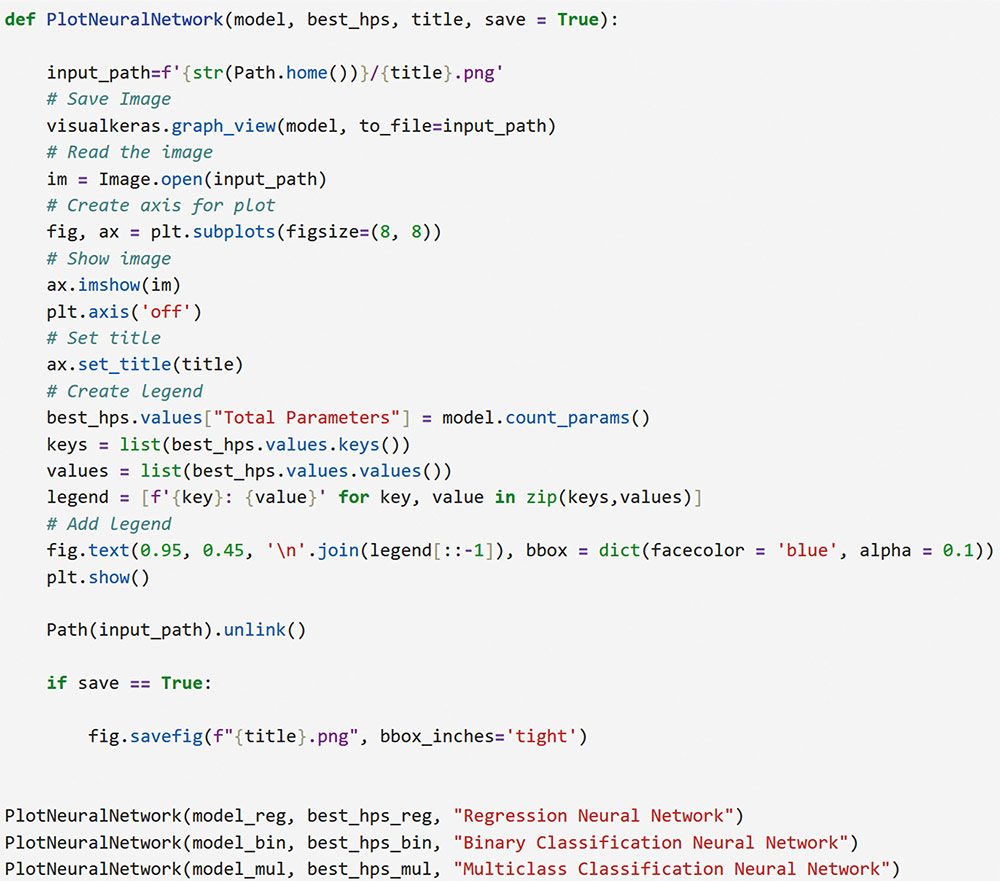 According to the execution of this script, the final model found for the regression task using MLP featured three layers. The first and second hidden layers each have 15 neurons with ReLU activation. The output layer consists of a single neuron, typical for regression, likely using a linear activation function. The model includes a learning rate of approximately .085, and a regularization strength of .049 to prevent overfitting. It has a total of 391 parameters which are the weights and biases of each layer (Figure 11). Figure 11 Regression Neural Network Architecture. 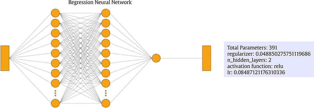 To check there was no overfitting during training, we plot the learning curves of the training process for the training and validation data. We define a function that takes the trained model and plots the loss and validation loss for each epoch on the same plot using the matplotlib plot function. We also pass the appropriate title as a parameter (Figure 12). Figure 12 Plotting Loss Curve for Each Task. 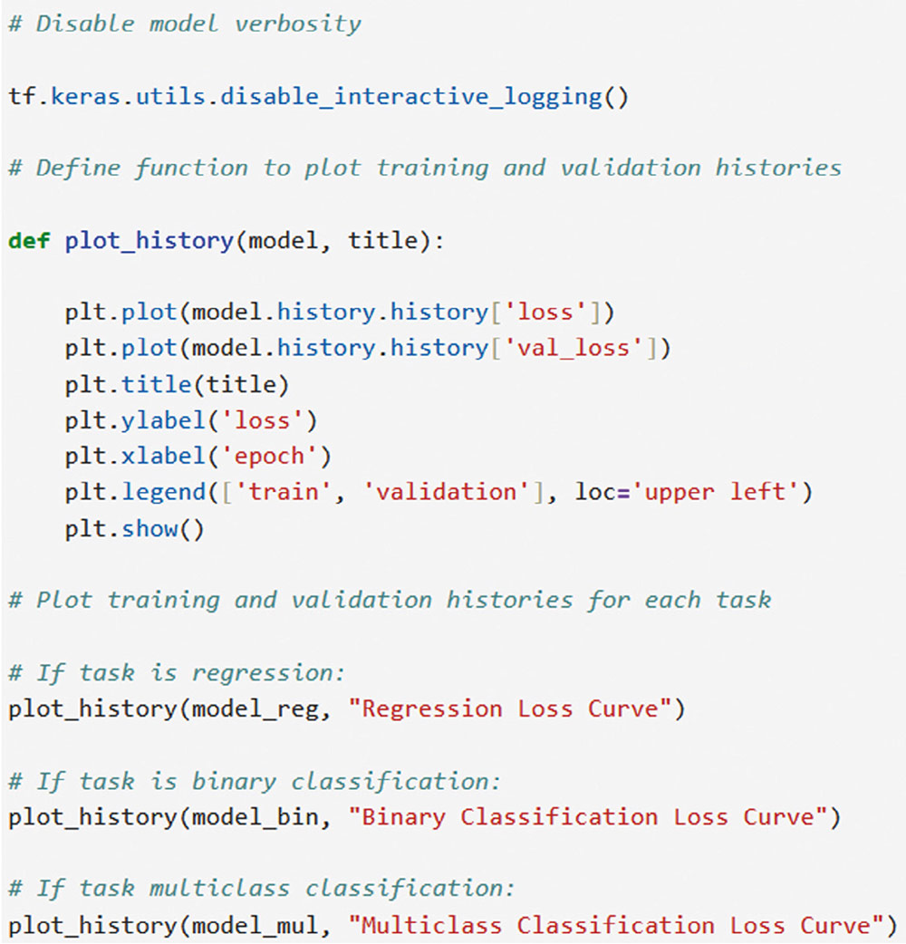 These are the loss curve plots for each task: regression, binary classification, and multiclass classification. A loss curve for a MLP shows how the model’s performance changes during training, with loss values on the y-axis and epochs on the X axis. It typically includes training loss, which decreases as the model learns, and validation loss, which reflects generalization to unseen data. In a well-performing model, both losses decrease and converge. If validation loss plateaus or increases while training loss decreases, it may indicate overfitting. The curve helps identify learning progress, diagnose issues like underfitting or overfitting, and determine when to stop training (Figure 13). Figure 13 Regression Loss Curve, Binary Classification Loss Curve and Multiclass Loss Curve. 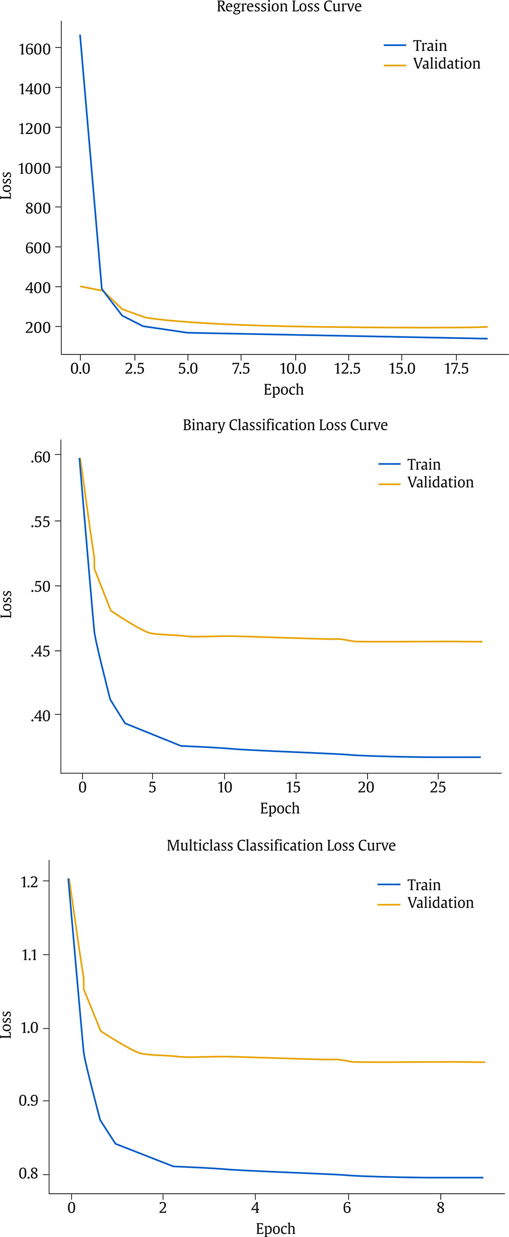 Assessment of Model Performance Regression Task Once the models have been trained, we can measure their performance using the test dataset. Although the training data can be used to gain an insight into the model fitness, it is not a reliable source of the model’s generalisation error due to its high complexity and thus risk of overfitting. However, as the test dataset was not used before, it is essentially new data the model has not seen. There is not a single metric that can capture the model’s performance so we will compute the most used and standard metrics in the literature like root mean square error (RMSE), mean absolute error (MAE), or R2 (see Supplementary Material for further details). To extract the predictions of the model from a given dataset, we define a function that perform the calculation of the regression metrics. We will compute the predictions of the model using the predict method on the model object and pass the data as a parameter. The results can then be presented in a table format by creating a pandas DataFrame with all the results. In our case, we compare the performance on the training, validation and testing data (Figure 14). Figure 14 Computing Regression Performance Metrics for Training, Validation and Test Datasets. 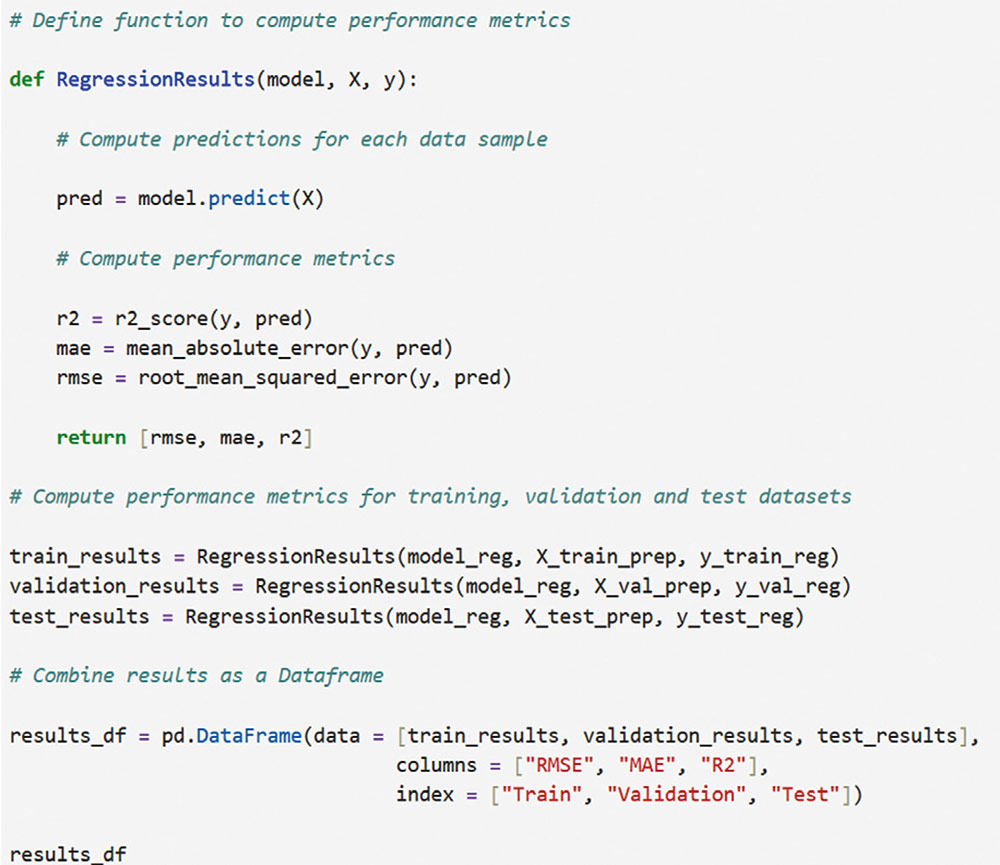 Once the script is executed, the MLP model’s performance is best on the training data, with the lowest RMSE (11.17) and MAE (8.86), and the highest R2 (.78). This is expected as the model is optimized on this dataset. Performance on the validation and test sets is slightly worse but relatively consistent. The validation set shows RMSE of 13.66, MAE of 11.22, and R2 of .64. The test set results are similar with RMSE of 13.27, MAE of 10.56, and R2 of .71. The consistency between validation and test results suggests good generalization. The R2 values indicate moderate to good predictive power, explaining 64-71% of the variance in the validation and test sets. The similar performance across datasets suggests the model is not overfitting significantly to the training data (Table 1). Table 1 Regression Performance Metrics. 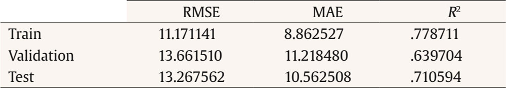 An important limitation of neural networks and other black box model compared to more classical linear models is their lack of interpretability. Over the last decade however, there has been an important line of research trying to tackle this limitation. A very common method to gain insights into the models’ inner workings is permutation importance of the features (input variables) which allows to gain a measure on the importance of a giving variable (or feature) in the models’ overall performance (see Supplementary Material for further details). We use sklearn implementation of the technique which requires the model itself as well as the data used for evaluation, which will normally be the testing data, and the metric used for measuring the models’ performance, which will usually be the RMSE for a regression problem. To pass the sklearn metric to the function we will have to first transform it to a scorer using the make_scorer function from the sklearn library. To present the results, we define a function which takes the output of the sklearn implementation and returns a plot showing the mean importance for each feature as well as the standard deviation. The function integrates into the graphical representation the quantitative values of computed variable importance, accompanied by their respective confidence intervals. The next script allows to create function (Figure 15). Figure 15 Permutation Feature Importance Plotting Function. 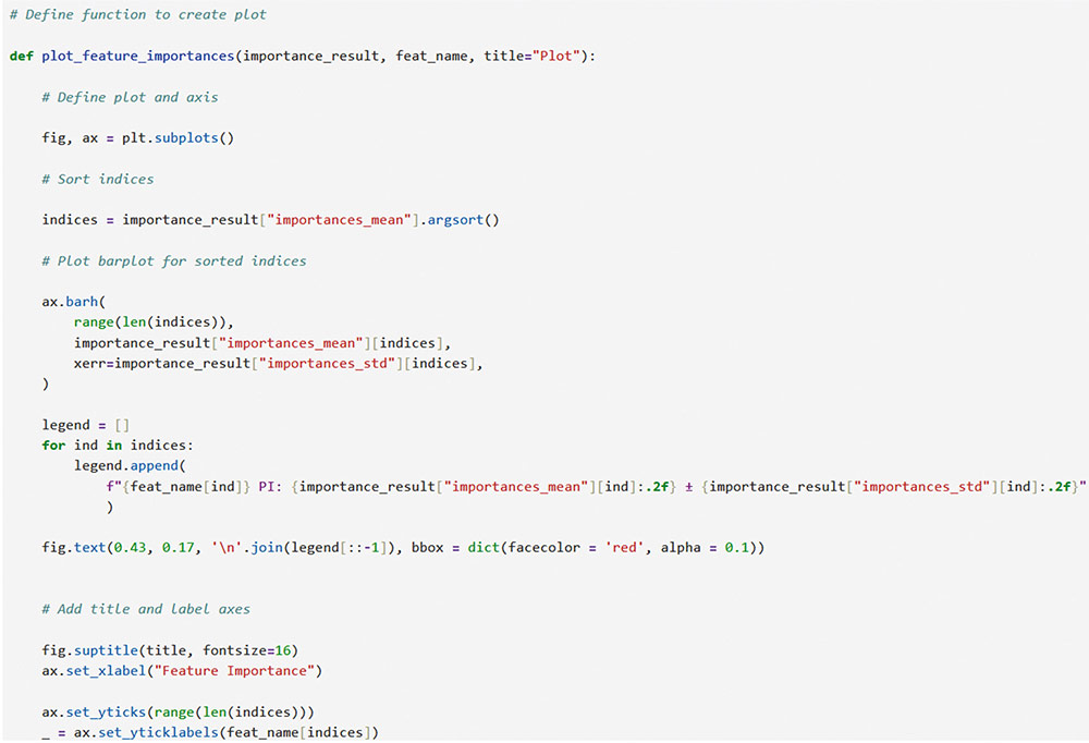 The permutation method for the regression task can be implemented using the following script using the function “permutation_importance”. When using permutation feature importance with RMSE as the scoring metric (and greater_is_better = False), the importance of each variable is expressed as the “increase in RMSE” caused by permuting that feature. Higher values indicate greater importance (Figura 16). Figure 16 Plotting the Permutation Feature Importance for Regression Task. 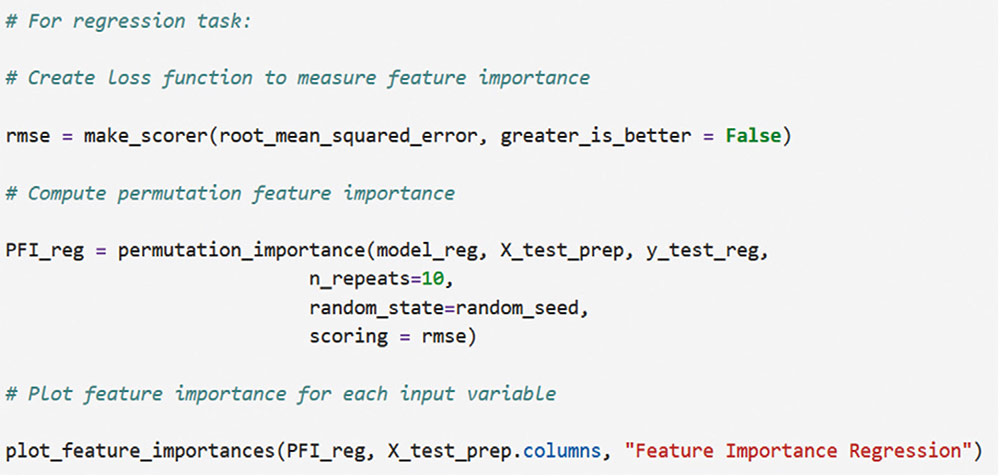 Figure 17 Feature Importance Regression. If you run the script, this is the plot of feature importance of the MLP for the task regression using the permutation procedure. The order of importance exactly reflects the simulated existing relationships in the dataset: Depression (-.80), Life satisfaction (.60), Emotional intelligence (.50), and resilience (.40). The importance of age (initially .15) is non-significant (.04 ± .05) and also socioeconomic status (Figure 17). The MLP model’s solution thus accurately captures the simulated relationships between the predictor variables and the response variable, effectively representing the underlying data structure. Classification Task For binary and multiclass classification tasks, predictions are obtained using the MLP model’s predict method. However, many classification metrics require discrete class labels rather than probabilities. In binary classification, a threshold (typically .50) is applied to determine class membership. To convert probabilities into class predictions, we can utilize the ‘where’ function from the “numpy” library. This function allows us to efficiently transform the continuous probability outputs into discrete class labels based on the chosen threshold. Model performance is evaluated using various metrics from the Sklearn library, comparing target and predicted classes. We focus on specificity, sensitivity, F1-score, AUC, and Cohen’s kappa score (see Supplementary Material for further details). A custom function will compute these metrics for training, validation, and testing datasets, with results presented in a DataFrame. The following script computes those metrics of the MLP binary classification task (Figure 18). Figure 18 Computing Binary Classification Performance Metrics. 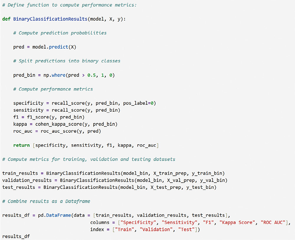 The MLP model exhibits robust performance in the binary classification task, as demonstrated by the metrics. Results for test set, which provide the most reliable assessment of the model’s ability to generalize to unseen data, reveal a specificity of .878, indicating a strong capacity to correctly identify negative instances. The sensitivity of .784 reflects a good ability to identify positive instances. The F1-score of .825 suggests a balanced performance between precision and recall. The Cohen’s kappa score of .661 signifies a moderate agreement between predicted and actual classes, exceeding what would be expected by chance alone. Critically, the high AUC of .926 on the test data confirms the model’s excellent ability to discriminate between the two classes (Table 2). Table 2 Binary Classification Performance Metrics. 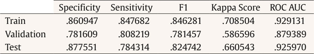 In classification tasks, results are often visualized using confusion matrices and ROC curves. Sklearn’s ConfusionMatrixDisplay and RocCurveDisplay facilitate this. We create a normalized confusion matrix using the “confusion_matrix” function, passing target and predicted classes as parameters. The resulting matrix is then visualized using ConfusionMatrixDisplay, with class labels from the OneHotEncoder. The plot method displays confusion matrices for training, validation, and testing data. Similarly, ROC curves can be plotted using RocCurveDisplay for each dataset. This is the script for obtaining the confusion matrices (Figure 19 and 20). Figure 19 Plotting Binary Classification Confusion Matrix. 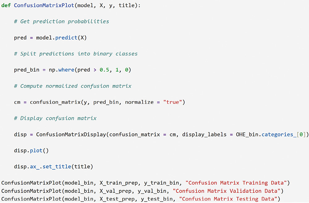 Figure 20 Confusion Matrix Training Data, Confusion Matrix Validation Data and Confusion Matrix Testing Data. 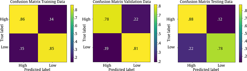 The MLP model’s confusion matrix on the testing data reveals good performance in classifying “High” psychological well-being (88% accuracy) but a tendency to misclassify “low” psychological well-being as “high” (22% error rate). While “high” classification is strong, “low” classification accuracy is lower (78%), and misclassification as “high” is more frequent than the reverse. This suggests a bias toward the “high” class, warranting potential model adjustments. The slightly worse results in the MLP binary classification task, compared to the regression task predicting psychological well-being as a continuous variable, stem primarily from the nature of the outcome variable rather than a deficiency in the MLP model itself. Dichotomizing the continuous well-being variable into “high” and “low” categories inherently discards nuanced information about the degree of well-being, which was available in the regression task. This loss of information makes the classification problem intrinsically more challenging, as the model must now discriminate between broad categories lacking the fine-grained distinctions present in the original continuous scale. Consequently, the observed difference in performance is largely attributable to the simplification of the outcome variable and the resultant loss of information, rather than an inherent limitation of the MLP architecture. The nature of the classification is such that it is harder than regression, even when the same model is used. To display the ROC curve, we first create the figure and axis of the plot using the subplots function from matplotlib library. We can then pass the target class as well as the probabilities belonging to each class to the “from_predictions” method of the RocCurveDisplay object as well as specify the axis on which the curve will be plotted. Finally, we can also set the colour and the label of each curve as well as set the axis labels and the title of the plot as follows (Figure 21). Figure 21 Plotting Binary Classification ROC Curves. 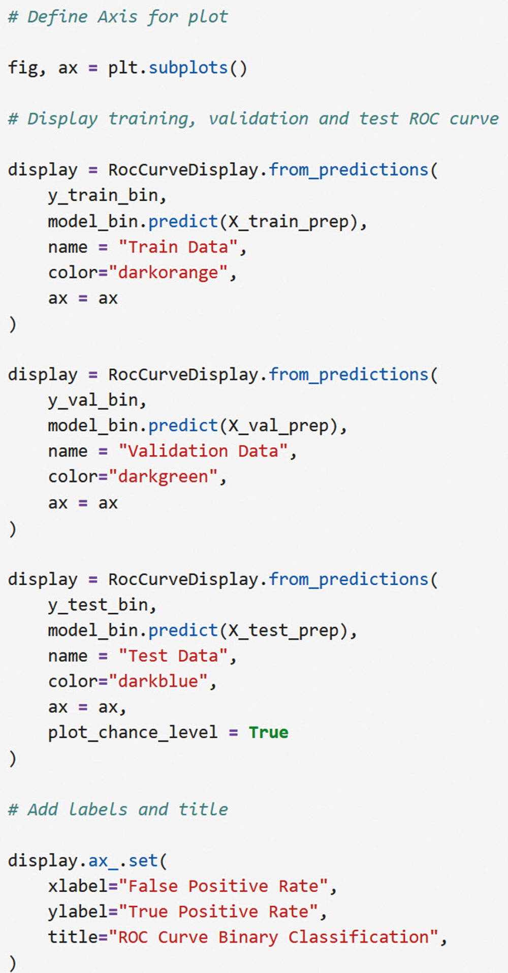 The MLP model achieves excellent discrimination between classes, as evidenced by the high AUC scores. The training and test datasets both reach an AUC of .93, indicating strong performance and generalization. The validation dataset, with a slightly lower AUC of .88, still demonstrates good discrimination ability. All AUC values are significantly above the chance level (.05), highlighting the model’s effectiveness (Figure 22). Figure 22 Binary Classification ROC Curves. 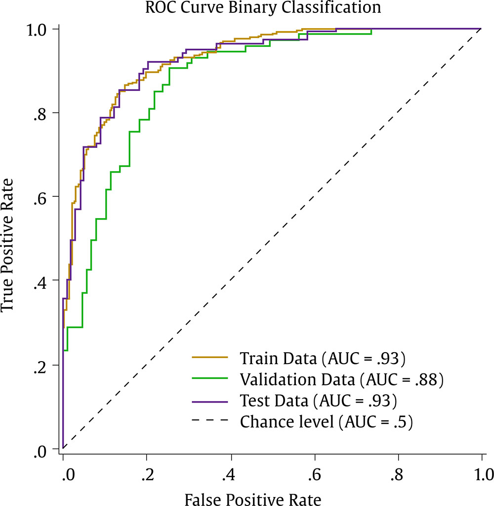 Finally, to measure the importance of each input variable we make use of the “permutation_importance” function again. However, we now use the AUC as the figure of merit to measure the model’s performance. To pass the Sklearn metric to the function we have to first transform it to a scorer using the “make_scorer” function from the Sklearn library (Figure 23). Figure 23 Plotting Permutation Feature Importance for Binary Classification. 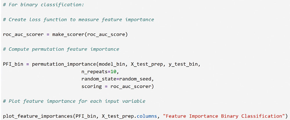 In this case, the Feature Importance values represent the decrease in AUC score when each feature is shuffled. Higher values indicate greater importance for class discrimination. Depression emerges as the most influential variable (.28 ± .04), while other features appear non-significant. The importance ranking largely aligns with the MLP regression task results, barring the non-significant influences (Figure 24). Figure 24 Feature Importance Binary Classification. 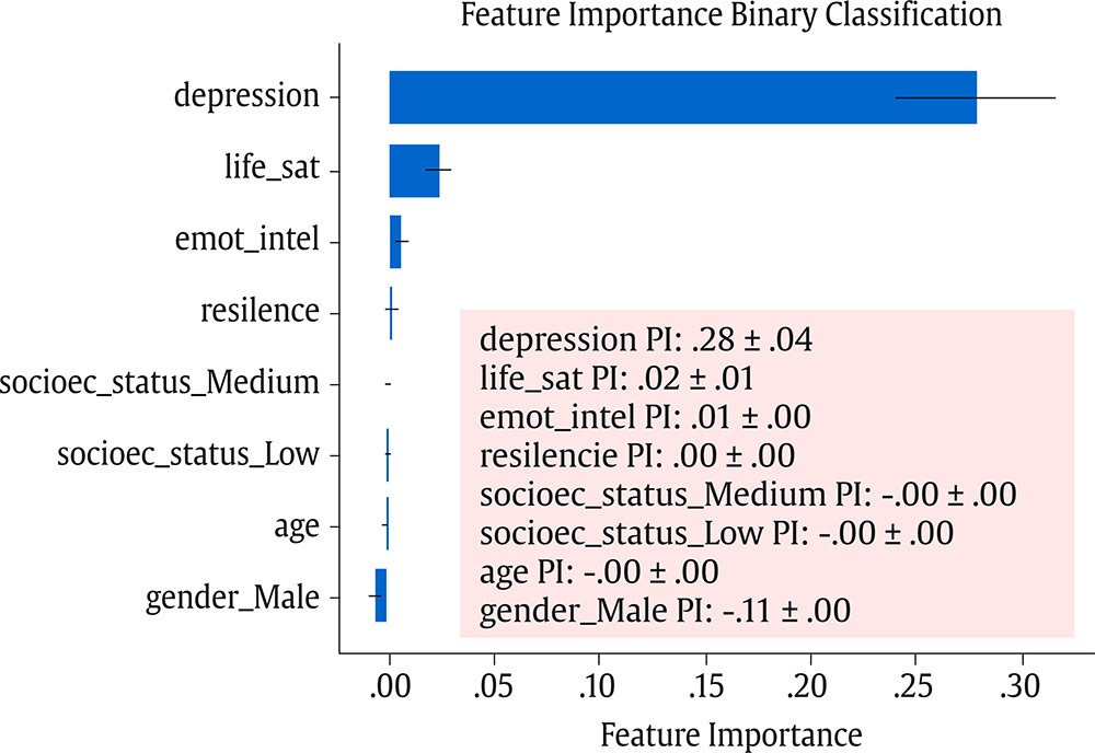 For the multiclass classification task, we adapt our approach to handle four classes instead of two. We use the “argmax” function from numpy to select the class with the highest predicted probability, then convert these indices to one-hot encoded values using keras’s “to_categorical” function. Unlike the binary case, many metrics don’t directly support multiclass values. We address this using a one-versus-rest approach, computing metrics for each class separately by treating it as positive and the others as negative. This process is implemented in a for loop, with results stored in pre-defined lists. The final results are presented in a pandas DataFrame, similar to the binary classification task, but now encompassing metrics for all four classes (Figure 25). Figure 25 Computing Multiclass Classification Performance Metrics. 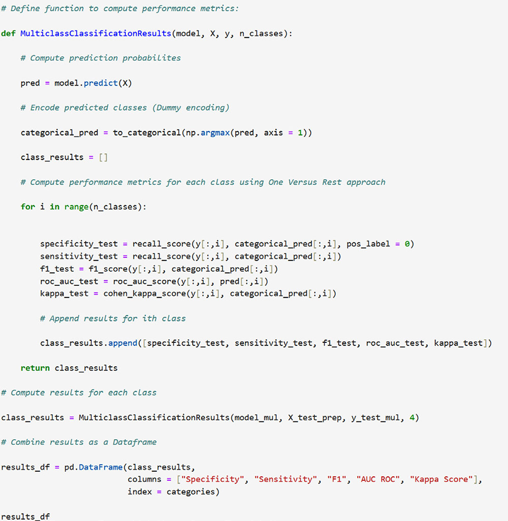 The MLP model’s test set performance reveals varying success across the four psychological well-being categories. The “low” and “very much” categories demonstrate superior discrimination, as evidenced by their high specificities (.969 and .930, respectively) and AUCs (.934 and .933). This likely stems from these categories representing the extreme ends of the underlying continuous psychological well-being scale, leading to clearer differentiation based on the input features. The somewhat and quite a bit categories, conversely, exhibit lower specificities (around 0.800) and AUCs (around .815), suggesting slightly poorer classification. The F1 and Kappa values confirm this mixed pattern. The poorer performance in the intermediate categories may be attributable to the artificial “fuzziness” introduced by the polytomization process of the continuous output variable in the simulated dataset, where these categories capture a more heterogeneous group of individuals, making them inherently more difficult to classify than the more distinct extreme categories (Table 3). Table 3 Multiclass Classification Performance Metrics. 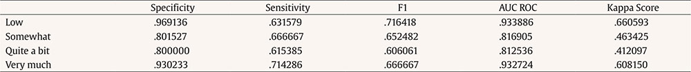 The process for generating the confusion matrix in the multiclass task closely mirrors that of the binary case. We use the same “confusion_matrix” function with normalized output and pass the resulting object to ConfusionMatrixDisplay. The key difference lies in the inclusion of all four category names, retrieved from the OneHotEncoder used in preprocessing, instead of just two. The plot method is then called to visualize the matrix, providing a comprehensive view of the model’s performance across all four classes (Figure 26). Figure 26 Plotting Confusion Matrix for Multiclass Classification. 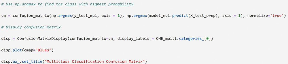 Figure 27 Multiclass Classification Confusion Matrix. 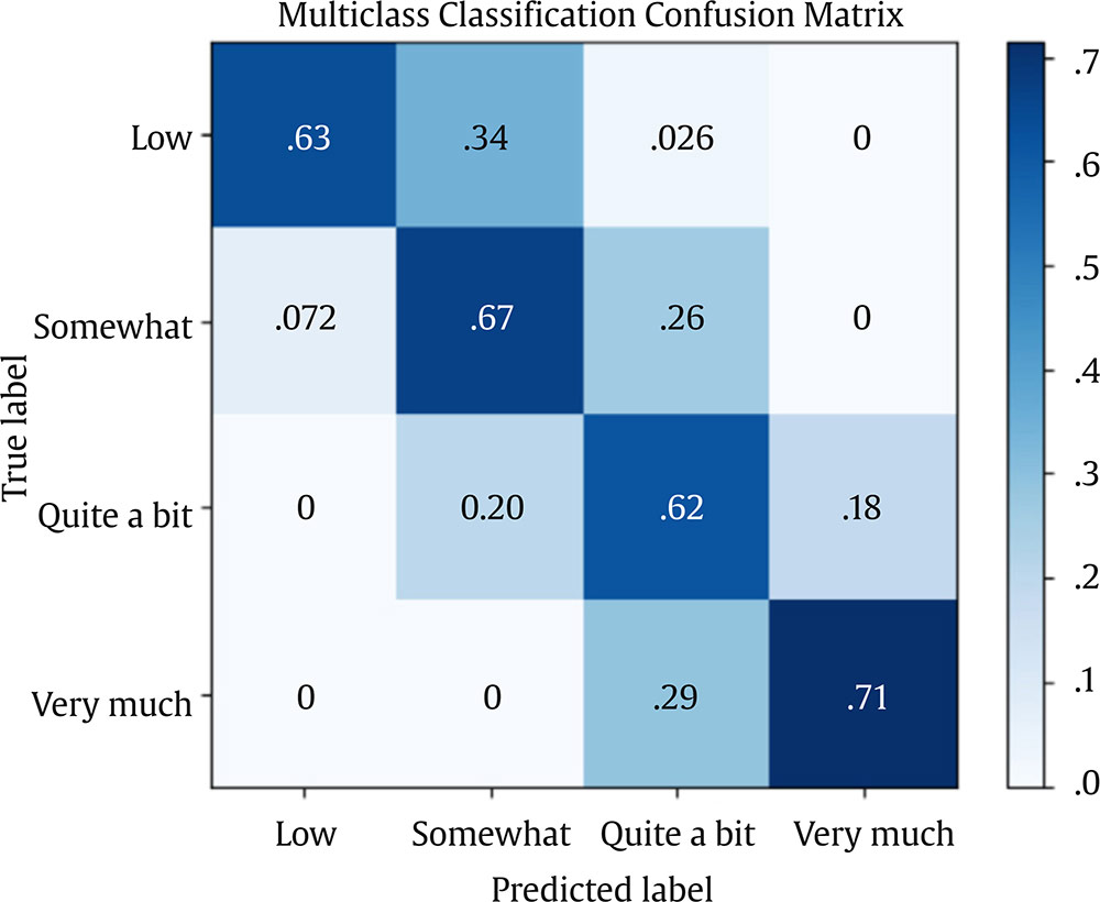 For conciseness, we only compute and present the confusion matrix for the test set, providing a focused evaluation of the model’s generalization performance. The MLP model achieves 71% accuracy in classifying “Very much”, and around 63-67% for the remaining classes. The primary challenge lies in differentiating adjacent categories. Notably, 34% of actual low instances are misclassified as somewhat; somewhat instances have a 26% chance of being misclassified as quite a bit, while 20% of quite a bit instances are misclassified as somewhat, and 18% of quite a bit instances are misclassified as very much. This indicates confusion between neighboring levels of psychological well-being, and a lower sensitivity when discriminating quite a bit instances (Figure 27). To create the ROC curve plot we need to use the one-versus-rest approach again and compute a ROC curve for each class separately. Therefore, when computing the ROC curve for the i’th class, we need to pass the i’th index of both the target outcome and the predicted probabilities to the RocCurveDisplay function. As this has to be repeated for each class, we will run the code inside a for loop and attach a different colour for each curve (Figure 28). Figure 28 Plotting ROC Curves for Multiclass Classification. 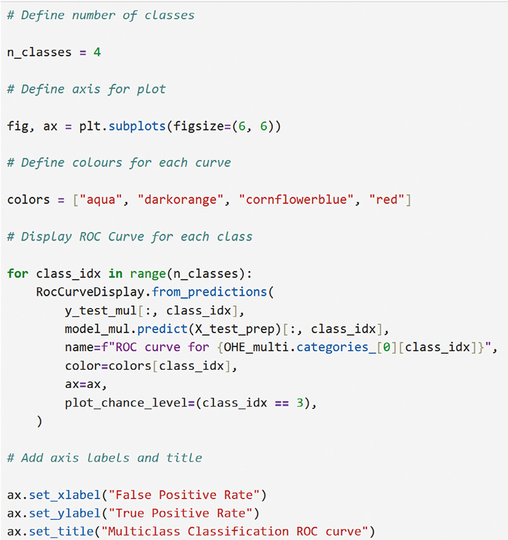 Figure 29 Multiclass Classification ROC Curve. 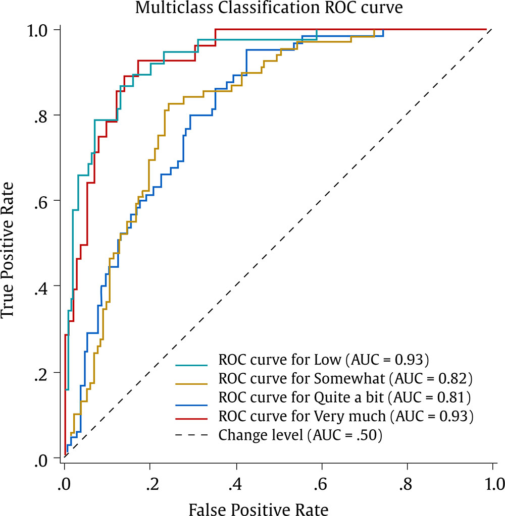 The model achieves its highest discrimination for the low and very much classes, both with an AUC of .93, while the somewhat and quite a bit classes have AUC values of .82 and .81, respectively (Figure 29). Finally, for the permutation feature importance we use the AUC as figure of merit and use the one-versus-rest approach. Thus, we will have four feature importance plots, one for each class. We set the average parameter to none and the “multi_class” parameter to ‘ovr’ inside the “make_scorer” function to compute the AUC for each class. We then extract the importance mean and importance standard deviation for each class from the results by accessing the i’th index for the i’th class. The results can then be plotted separately as the following script includes. Again, for conciseness, we only display the ROC curves for the test set (Figure 30). Figure 30 Plotting Permutation Feature Importance for Each Class. 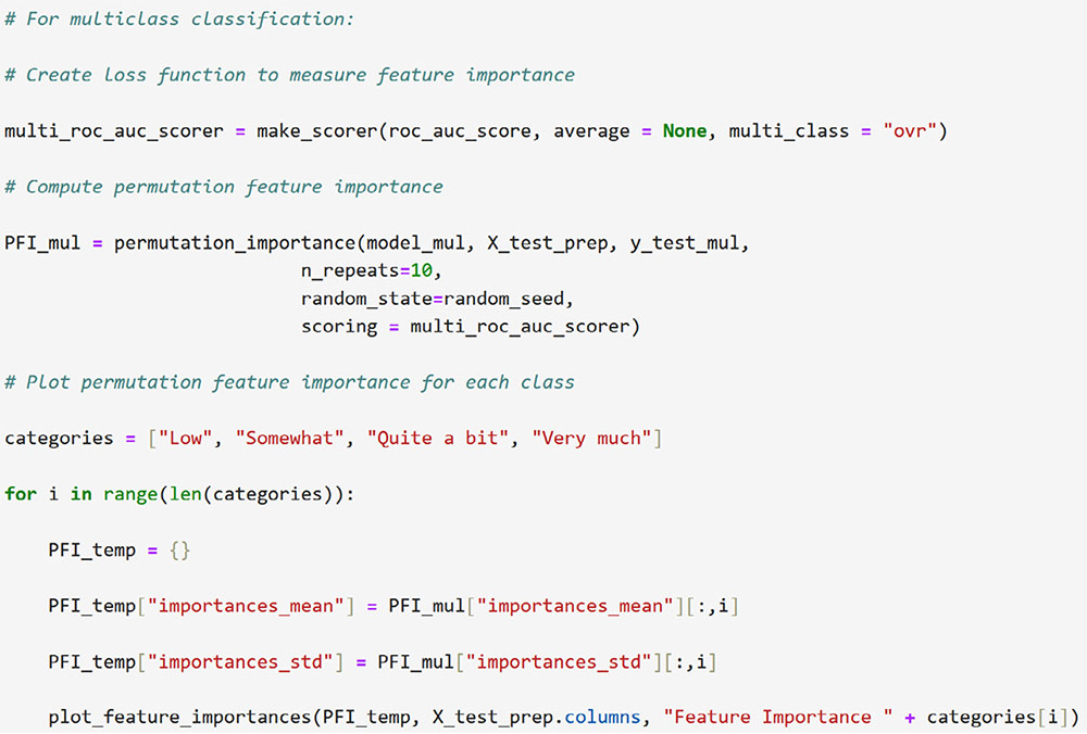 The importance plot based on the permutation method reveals a similar structure across all four classes. Depression emerges as the most important variable in every case, with values ranging from .22 (quite a bit) to .26 (very much). The solutions also converge on the second most important variable, Life Satisfaction, which ranges from .02 to .06. The remaining input variables exhibit virtually negligible importance (Figure 31). Figure 31 Feature Importance Plots for Multiclass Classification. 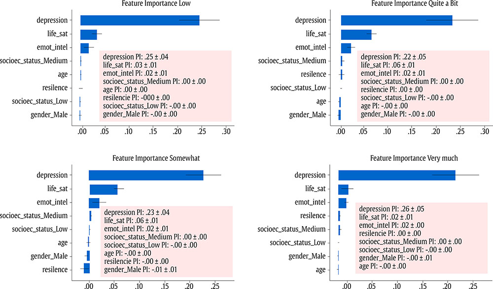 In this tutorial, we have shown the flexibility of a MLP by applying the same general Python script, adapted to different predictive tasks: regression, binary classification, and multiclass classification. By using “psychological well-being” consistently across tasks, first as a continuous variable for regression, then dichotomized for binary classification, and finally polytomized for multiclass classification, we ensured direct comparability of the results. For each task, we computed the appropriate evaluation metrics and visualized the outcomes through relevant plots, providing a comprehensive view of the model’s performance in different predictive scenarios. Beyond showcasing the applications of MLP, our goal was to illustrate the implementation and interpretation of these models in an accessible way. By systematically presenting the Python scripts and the corresponding analyses, we aimed to demystify the use of ANNs in Behavioral and Health Sciences research. The complete script with the three tasks and a separate one for each task can be downloaded in the following links: all tasks compiled (link 4), regression task (link 5), binary classification task (link 6), and multiclass classification task (link 7). Our learning objective and optimal strategy is to enable readers to execute all analyses, verify results, and alleviate anxiety potentially associated with the use of programming languages in statistical modeling. We assure the reader that the experience is highly rewarding, particularly for researchers who, in general, are not familiar with the models at the core of AI, nor specifically work regularly with platforms that operate using programming languages. For this reason, we hope this work serves as a practical guide for researchers unfamiliar with these AI models, encouraging them to incorporate MLPs into their methodological toolkit and expanding the range of analytical approaches available for their studies. Conflict of Interest The authors of this article declare no conflict of interest. Cite this article as: Martínez-García, J., Montaño, J. J., Jiménez, R., Gervilla, E., Cajal, B., Núñez, A., Leguizamo, F., & Sesé, A. (2025). Decoding artificial intelligence: A tutorial on neural networks in behavioral research. Clinical and Health, 36(2), 77-95. https://doi.org/10.5093/clh2025a13 Funding This study has been supported through the funded recruitment project 2023-24_8_61 RI-24, thanks to the Recovery and Resilience Mechanism Funds (EU - Next Generation) involving the European Union, the Ministry of Labour and Social Economy (Spain), the Autonomous Government of the Balearic Islands and the University of the Balearic Islands. Dataset, supplementary material and Python scripts can be found at the following links:
References | Introduction The Multilayer Perceptron (MLP) and the Backpropagation Learning Algorithm: The Most Prevalent ANN Objectives of the Tutorial Dataset Generation Software and Platform Setup Steps in the Application of an MLP in Regression and Classification Tasks Importing Required Libraries Calling the Data Matrix and Selection of Variables Creation of Training, Validation and Test Sets Data Pre-processing Neural Network Model Design Training the Final Model Assessment of Model Performance Conclusions data-availability |
Cite this article as: Martínez-García, J., Montaño, J. J., Jiménez, R., Gervilla, E., Cajal, B., Núñez, A., Leguizamo, F., and Sesé, A. (2025). Decoding Artificial Intelligence: A Tutorial on Neural Networks in Behavioral Research. Clinical and Health, 36(2), 77 - 95. https://doi.org/10.5093/clh2025a13
Correspondence: juanjo.montano@uib.es (J. J. Montaño Moreno).Copyright © 2026. Colegio Oficial de la Psicología de Madrid


 PDF
PDF e-PUB
e-PUB CrossRef
 JATS
JATS Print
Print Send
SendEMAIL ALERT
Clinical and Health is licensed under a Creative Commons Attribution-NonCommercial-NoDerivatives 4.0 International License