Procedures for Comparison of Two Means in Independent Groups with R
Alfonso Palmer, Albert Sesé, Berta Cajal, Juan J. Montaño, Rafael Jiménez y Elena Gervilla
University of the Balearic Islands, Spain
https://doi.org/10.5093/clysa2022a1
The comparison of two means in independent groups is one of the most used statistical procedures. In the bibliometric study carried out by Sesé and Palmer (2012) on the 623 articles published in 8 impact journals of Clinical and Health Psychology, in 2010, it was found that the parametric comparison of two means in independent groups was the second most used statistical technique (n = 161 times) only surpassed by correlation (n = 207), while non-parametric techniques in general (n = 54), resampling (n = 12), and robust (n = 4) were in descending order. However, only 17.27% of the articles evaluated the assumptions of the procedure used, failing the rest in one of the fundamental aspects of statistics. The objective of this work is to show different procedures that should be used depending on the scenario in which the data analysis is found. In this analysis we have a categorical variable, which can be binary or a factor with k = 2 levels and a vector of continuous responses. This information can be entered into R by two data vectors. Below are provided, as an example, the fictitious responses of 12 subjects belonging to each of the two groups: 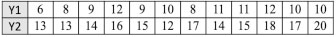 Speaking in generic terms, vectors Y1 and Y2 can correspond to an experimental group and a control group, to two experimental conditions, to responses of men and women, etc. In terms of R, the two response vectors are defined: > Y = c(6, 8, 9, 12, 9, 10, 8, 11, 11, 12, 10, 10) > Y2 = c(13, 13,14, 16, 15, 12, 17, 14, 15, 18, 17, 20) A vector, called Y, is generated that joins both vectors Y1 and Y2. Y = c(Y1,Y2) > Y [1] 6 8 9 12 9 10 8 11 11 12 10 10 13 13 14 16 15 12 17 14 15 18 17 20 The dichotomous variable Grupo is generated, which defines which group each response corresponds to and which differentiates the responses of vector Y1, with a value of 0, from the responses of vector Y2, with a value of 1. Grupo = as.factor(c(rep(0,12),rep(1,12))) > Grupo [1] 0 0 0 0 0 0 0 0 0 0 0 0 1 1 1 1 1 1 1 1 1 1 1 1 Levels: 0 1 Finally, a data matrix that will be named Data is created, with two columns: the first is the Y vector and the second is Grupo. > Datos = data.frame(Y, Grupo) The sample means of the two groups are obtained, which allow the comparison of the two population means, as well as the difference of the sample means: 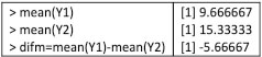 The box plot of the two distributions is displayed using the ggplot function of the ggplot2 library: 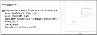 The following is a non-exhaustive overview of the different scenarios in which a researcher may find himself having to make a comparison of two means in independent groups and of the procedures to use, with R, in each scenario. The syntax in R and the most relevant results are provided. A broader description and the formulas on which each test is based can be found in Palmer (2011), while practical applications, with R, can be found in Palmer (2013) and Palmer (2019). Assumptions. Parametric tests require the fulfillment of some assumptions, that in the case of a comparison of two means in independent groups refer to normality and equality of variances (homoscedasticity) in the original populations of both groups. These conditions of application are evaluated below: 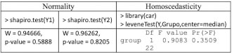 Thus, the Shapiro-Wilk test allows us to conclude the null hypothesis of normality in the original populations of both groups, while the robust Levene test maintains the null hypothesis of equality of population variances. It should be remembered that the evaluation of the assumptions must always be carried out and, based on its results, a correct decision can be made about the procedure to follow. t test. The parametric test to use when both assumptions are met, is the Student’s t-test. In this case, in addition to providing the test value and its degree of significance (p-value), the APA recommends also providing the confidence interval, generally 95%, (Palmer y Sesé, 2013). 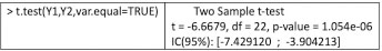 Linear regression model. Equivalently to Student’s t, the linear regression model can also be applied, but in this case using the lm function: 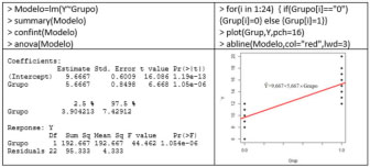 The Grupo coefficient is the difference of means. In this case, when moving the Grupo from 0 to 1, the mean of Y increases 5.667, so it appears with a positive sign. For this reason, the CI (95%) appears with a change in sign to that of the t-test, but they are equivalent. Model comparison. In this case, the model comparison consists in comparing the predicted value of Y with (extended model) or without (reduced model) the Grupo variable. The comparison of models is applicable to the parametric way and its results are equivalent to the t-test. The following table shows the application to the parametric way: 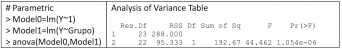 Welch test. If the homogeneity of variance is not satisfied, then the Welch test is used, which is a Student’s t-test with a modification in the degrees of freedom: 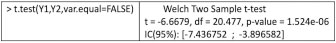 Weighted linear model. Under non-equality of variances, the weighted linear model can be used, where the weight of each observation is the inverse of the variance of the group to which it belongs. The weight affects the value of the standard errors.  Sample size, effect size and power. Some important elements in a hypothesis test have to do with the sample sizes of each group, the size of the effect and the Power of the statistical test. All of these elements are related to each other, together with the alpha risk used (generally the value .05) and the type of test used (two-tailed or one-tailed). Effect size is a standardized measure of the difference between means. A very popular measure is Cohen’s (1988) d, which can be obtained using the cohen.d function from the effsize library:  Cohen differentiates between small (d = 0.20), medium (d = 0.50) and large (d = 0.80) effect sizes, although it is better to interpret it in terms of percentiles (Palmer, 2011). With a Cohen’s d of 2, 97.7% of the “treatment” group will be above the mean of the “control” group (Cohen’s U3), 31.7% of the two groups will overlap, and there is a 92.1% probability that a person chosen randomly from the treatment group will score higher than a person chosen randomly from the control group (superiority probability). In the following link, https://rpsychologist.com/cohend/, entering the value of the index d obtained (the maximum is 2), the values and the above mentioned interpretations are provided. The power of the statistical test is the probability of rejecting the null hypothesis when it is false. The APA recommends always providing this term (American Psychological Association [APA, 2010]) Its value can be obtained using the pwr.t2n.test function from the pwr library. 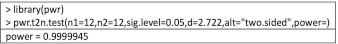 If the alternative hypothesis is one-sided, it will be enough to change the parameter alt = “less” or alt = “greater”. The power obtained is very high (0.99). If a low power is obtained, for example 0.22 when obtaining a d = 0.593 and the power of the test is to be increased to a certain value, the minimum sample size to use should be found. This minimum value of n, for each group, can be obtained with the pwr.t.test function, entering, among others, the value of the desired power, for example 0.80: 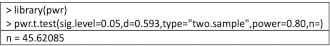 Therefore, to have a power of 80%, the size of each group should be at least n = 46. When the assumption of normality is not fulfilled, a non-parametric test can be used. In these tests, the original data is transformed into order numbers. Wilcoxon-Mann-Whitney test. One of the most common tests is the so-called Mann-Whitney U, also known as Wilcoxon-Mann-Whitney. It can be obtained through the wilcox.test function:  Linear regression model. The linear regression model can be applied, equivalently to the U test, in the non-parametric way, transforming the original values by their order numbers and applying the lm function: 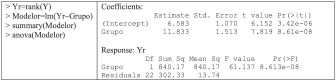 Model comparison. The comparison of models is applicable to the non-parametric route, its results being equivalent to the Mann-Whitney U test. To apply it in the nonparametric way, the vector Y must be transformed into order numbers, which is achieved with the rank function: 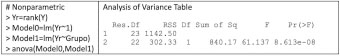 Robust test. When normality is not fulfilled and, above all, when there are “outlier” values, a robust test should be used, which uses a robust statistic instead of the mean (see Palmer, 1999). Yuen test. The Yuen test uses the trimmed mean. This test can be obtained with the yuen.t.test function from the PairedData library which by default cuts 20%: 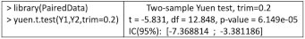 You can also get a bootstrap version of the Yuen test, with the yuenb function from the WRS2 library: 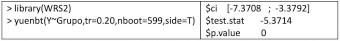 Compare M-estimators. A comparison of two M-estimators can be made instead of comparing two means using the pb2gen function of the WRS2 library. The final values of the Huber M-estimators are:  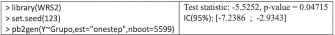 In this case, this function uses the value of the first iteration of the M-estimator Exact test. With small samples or when population distributions are unknown, resampling techniques, such as bootstrap or permutations procedures, can be used. For example, with the boot.ci function of the boot library, different formats of the CI (95%) can be obtained, while with the oneway_test function of the coin library, the exact Fisher-Pitman permutations test can be obtained:  Below are the results of the p-value for each of the statistical tests used. As can be seen, all the tests reach the same conclusion: The alternative hypothesis (p-value < .05) according to which there are significant differences between the two analyzed means can be accepted (see Table 1). Table 1 p value for Each of the Statistical Test Used  Also, this can be verified by seeing that the confidence intervals do not contain the value zero. The most important thing is to use the best procedure in each case based on the circumstances that arise. In the example presented, when the application conditions are met, the most powerful procedure to choose would be the parametric route. As there is normality, the non-parametric way is not required. As there are no outliers, the Robust way is not required, and although the exact way can be used, as it is small samples, in this case the parametric way is more powerful. In this example, all the procedures provide similar results since the conditions of application are met which will not happen when any of the assumptions are not fulfilled. The diagram in the following page provides an overview of the content explained in this article (Figure 1). Figure 1 Comparison of two Means in Independent Groups. 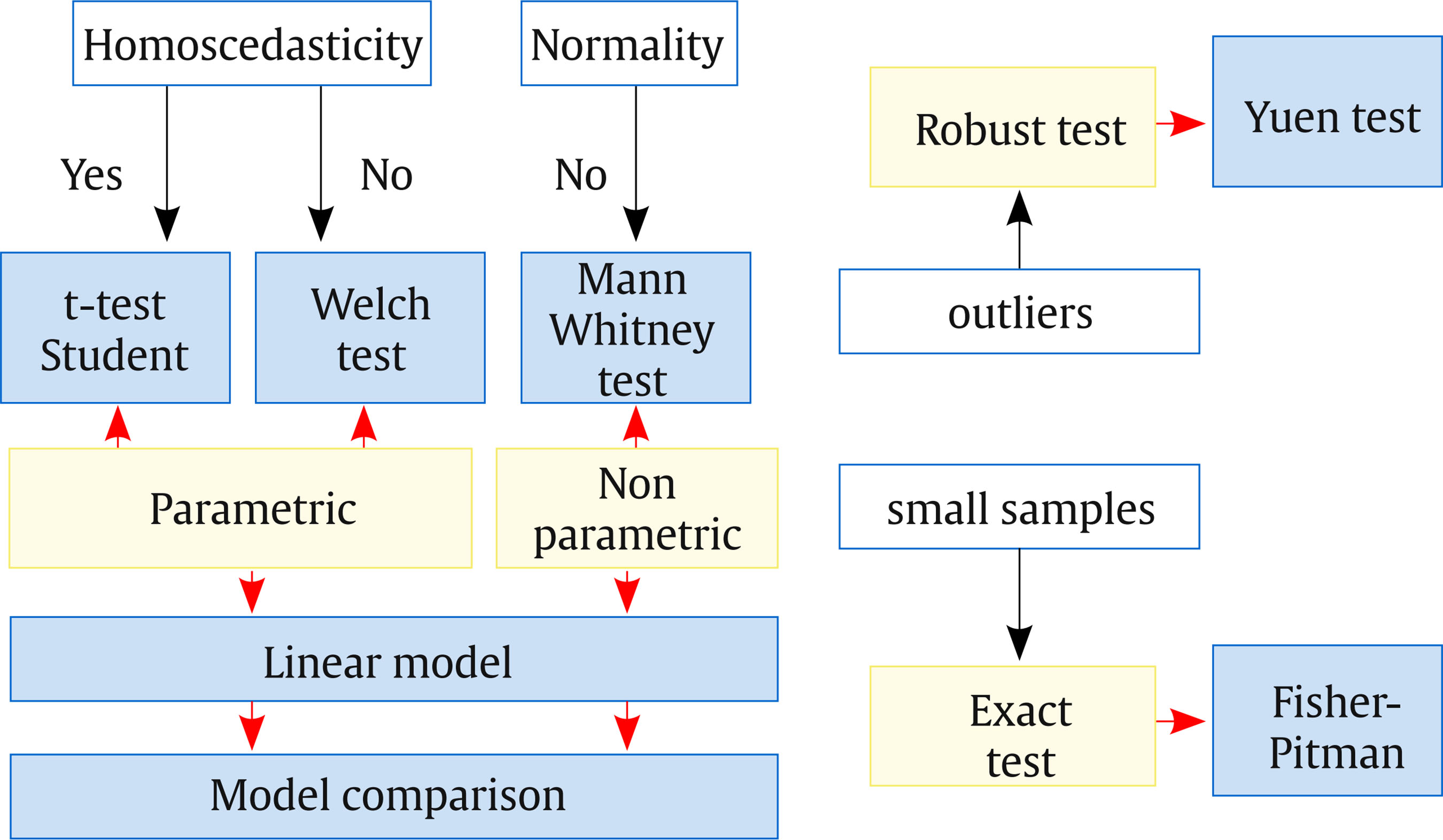 Cite this article as: Palmer, A., Sesé, A., Cajal, B., Montaño, J. J., Jiménez, R., & Gervilla, E. (2022). Procedures for comparison of two means in independent groups with R. Clínica y Salud, 33(1), 45-48.https://doi.org/10.5093/clysa2022a1 References |
Para citar este artÃculo: Palmer, A., Sesé, A., Cajal, B., Montaño, J. J., Jiménez, R. y Gervilla, E. (2022). Procedures for Comparison of Two Means in Independent Groups with R. ClÃnica y Salud, 33(1), 45 - 48. https://doi.org/10.5093/clysa2022a1
alfonso.palmer@uib.es Correspondence: alfonso.palmer@uib.es (A. Palmer).Copyright © 2026. Colegio Oficial de la Psicología de Madrid


 PDF
PDF e-PUB
e-PUB CrossRef
 JATS
JATS Print
Print Send
SendEMAIL ALERT
Clinical and Health is licensed under a Creative Commons Attribution-NonCommercial-NoDerivatives 4.0 International License